A famous problem in approximation theory is to approximate the function \left|x\right| as accurately as possible on the interval -1 \le x \le 1, measured by maximum absolute error, using either polynomials or rational functions of fixed degree.
Content Preview
A famous problem in approximation theory is to approximate the function
\left|x\right|
as accurately as possible on the interval
-1 \le x \le 1
, measured by maximum absolute error, using either polynomials or rational functions of fixed degree.
Perhaps it seems silly to approximate a function as simple as this, but it serves as a useful test problem for probing how well non-smooth functions can be approximated by polynomial or rational functions.
Polynomials can converge only linearly in their degree here, which we will call the “Bernstein bound,” and rationals can converge root-exponentially in their degree, which we will call the “Newman bound.” (The notation
E
refers to the
minimax
error — the smallest achievable maximum absolute error over the interval.)
The previous
two
posts
explored repeated composition of low-degree polynomials, which can generate polynomials of exponentially high degree in the number of operations. What happens when we apply this to the problem above?
In particular, consider Newton’s iteration for the inverse square root,
which can be derived by applying Newton’s method to the function
f(y)=1/y^2-x
. This iteration evaluates a polynomial of degree
\left(3^n-1\right)/2
in
x
using
3n
multiplications and
n
additions. To simplify a bit, we’ll consider a multiply followed by an addition as a
single operation
and say each iteration requires 3 “operations.” The absolute value follows from the inverse square root through
|x|=x^2\cdot(1/\sqrt{x^2})
.
Here is a plot showing the absolute error in this approximation, starting from
y_0 = 1
, for 10, 20, 30, 40, and 50 iterations:
x
abs. err.
The steady march of these curves on a log-log scale shows that as the number of iterations increases, the maximum error occurs at exponentially decreasing values of
x
and
decreases exponentially with iterations
.
The following table gives the maximum absolute error read from each of these curves.
iterations
operations
max. abs. error
10
30
4.7 × 10
-3
20
60
8.1 × 10
-5
30
90
1.4 × 10
-6
40
120
2.5 × 10
-8
50
150
4.3 × 10
-10
Fitting this data to an exponential
gives a very good fit with about 0.18 decimal digits of accuracy added per iteration (0.059 digits per operation).
This is exponential convergence in operation count — a qualitatively different rate than either the Bernstein or Newman bounds.
The rate constant, however, is somewhat low for practical purposes. The crossover points when comparing this Newton iteration against minimax polynomials and rationals of fixed degree on a per-operation basis are, respectively, 23 operations (max. abs. err. ≈ 1.2 × 10
-2
) and 217 operations (max. abs. err. ≈ 5 × 10
-14
). Newton iteration is a clear win over minimax polynomials of fixed degree, but only a win over minimax rationals of fixed degree if you need relatively high precision.
But this isn’t yet a fair comparison. The Newton iteration is not specifically optimized for this problem (i.e. for this approximation interval and error metric) at all, whereas the minimax polynomials and rationals have many optimized coefficients. What might be possible with optimized coefficients at each iteration?
The Bernstein bound still sets a limit here. After
n
iterations (
3n
operations), a Newton-like method with optimized coefficients would still evaluate a polynomial of degree
\left(3^n-1\right)/2
. Using this degree in the Bernstein bound implies exponential convergence with a maximum rate constant of log
10
(3) ≈ 0.48 digits per iteration (0.16 digits per operation). Perhaps surprisingly, the unoptimized Newton iteration is already within a factor of about 2.7 of this hypothetical optimum rate. If this rate were achievable, it would move the crossover points with minimax polynomials and rationals of fixed degree down to 8 operations (max. abs. err. ≈ 4 × 10
-2
) and 71 operations (max. abs. err. ≈ 3 × 10
-12
) respectively.
Further improvement may be possible by considering iterated
rational
maps, which can also evaluate rationals of exponentially high degree in the number of operations. Combining that observation with the Newman bound suggests that super-exponential convergence in operation count could be possible.
After some early experiments, I have not yet observed such super-exponential convergence, and I have doubts that it will in fact be possible. Consider, for example, Heron’s method for approximating square roots,
which can be derived by applying Newton’s method to the function
f(y)=y^2-x
. This iteration evaluates a rational function of type
(2^{n-1},\, 2^{n-1}-1)
after
n
iterations, using 3 operations per iteration (counting division as one operation). Using this iteration to approximate the absolute value through
|x|=\sqrt{x^2}
, starting with
y_0 = 1
, the maximum absolute error always
appears
to occur at x=0. This makes the error particularly easy to analyze: it is
2^{-n}
after
n
iterations. Exponential convergence, with rate constant 0.30 decimal digits per iteration (0.10 digits per operation). This is faster than the polynomial inverse square root iteration above, but not super-exponential.
How might this be improved with optimized coefficients per iteration? The Newman bound on degree, suggesting that super-exponential convergence in operation count may be possible, seems unlikely to be realizable to me, but I don’t yet know a lower bound than that.
I have suggested optimizing coefficients in polynomial and rational iterations. This is likely to be a challenging optimization problem because the maximum absolute error is a highly nonlinear function of these coefficients. However, I see some reason for optimism. Polynomial and rational iterations of the type I am describing are very similar to the layers of neural networks, and in fact, there has already been substantial research on polynomial neural networks. When compared to the neural networks that are being trained successfully for machine learning and artificial intelligence, the iterations I am describing are very small networks.
The central observation of this post is simple: the classical convergence rates for polynomial and rational approximation are stated in terms of degree, but degree is not the same as computational cost. When measured by operation count, iterated polynomial maps can achieve exponential convergence for problems where fixed-degree polynomials converge only linearly and fixed-degree rationals converge only root-exponentially. Exploring the full potential of this approach is an active area of research.
At this stage, I have many more questions than answers, and I will close with a list of them:
We have seen that Newton’s iteration for the inverse square root achieves full exponential convergence in operation count for the problem of approximating
\left|x\right|
on the interval
-1 \le x \le 1
by a polynomial. There is a factor of 2.7 gap between the rate constant realized by this technique and the maximum possible rate constant set by applying the Bernstein bound to the degree. Is it possible to achieve the full Bernstein bound? This would be surprising, in a way, since these iteratively generated polynomials have exponentially fewer coefficients than a polynomial in standard form of the same degree. But if the limit is lower, what is it?
Is super-exponential convergence in operation count possible for iterated rationals in this problem? If not, what is the maximum possible exponential convergence rate?
How generically can iterated polynomials and rationals approximate non-smooth functions with exponential (or super-exponential) convergence in operation count? The iterations we have examined are specific to approximating the square root and inverse square root, but similar iterations with optimized coefficients should be applicable more generally in principle. What performance can they achieve, say for the problem of approximating
|x|^{\alpha}
on
-1 \le x \le 1
for other positive
\alpha
?
Minimax
polynomial
and
rational
approximations are widely used in standard library implementations of mathematical functions, but almost always over intervals where the functions they approximate are smooth. Could iterated polynomials or rationals with optimized coefficients offer practical advantages in these settings?
Update 29 March, 2026
I shared this post with L. N. Trefethen who was kind enough to reply with some references. Composite polynomial and rational approximation is a more active area of research than I realized.
Trefethen’s short essay, “
Is Everything a Rational Function?
” discusses the idea of composing low-degree rational functions to evaluate exponentially high degree rational functions.
E. Gawlik and Y. Nakatsukasa, “
Approximating the pth root by composite rational functions
,” J. Approx. Theory, 2021, shows that super-exponential convergence (and in fact, fully double exponential convergence) in operation count
is
possible for iterated rationals applied to this problem. Wow! This fully answers my question 2 above, and goes a significant way toward answering my question 3 about how generic this convergence is by considering
x^{1/p}
for other integer
p
.
K. Yeon, “
Deep Univariate Polynomial and Conformal Approximation
,” arXiv:2503.00698, 2025, analyzes the same Newton inverse square root polynomial iteration that I considered in this post, reporting the same exponential convergence. The idea of using this iteration this way is credited to Jean-Michel Muller by private communication.
N. Boullé, Y. Nakatsukasa, and A. Townsend, “
Rational neural networks
,” Adv. Neural Info. Proc. Syst., (2020), discusses rational neural networks, which appear to be equivalent to composite rational functions. I think the difference is largely size and application.
Matrix squaring can also rapidly sum the geometric series
Let
a_n
and
b_n
denote the upper-left and upper-right entries of
M^{2^n}
. Writing the result of squaring the matrix shows that they satisfy the recurrence
Since
b_n = S_{2^{n}-1}(x)
, this recurrence allows computing
S_{2^{n}-1}(x)
with
2n
multiplications and
n
additions: exactly the same operation count as the Newton iteration discussed in
yesterday’s post
.
The matrix squaring iteration is connected to the Newton iteration by the identity
a_{n} = 1 - (1-x)b_n = x^{2^n}.
This allows writing a recurrence for
b_n
alone,
b_{n+1} = b_n(2 - (1-x)b_n),
which is exactly the Newton iteration from yesterday (where it was written using the variable
y_n
).
The two iterations—matrix squaring, and the Newton iteration—compute identical results (in exact arithmetic) with identical operation counts, but they are not quite identical computationally. They operate on different state spaces: the Newton iteration operates on a single number, and the matrix squaring iteration operates on a pair of numbers.
They also arrange their multiplications and additions differently, so that in floating point arithmetic, they have different numerical stability. I claim that the Newton iteration is more numerically stable in the region where the series converges,
-1\lt x\lt 1
, but I won’t go into further detail today.
Newton's method can rapidly sum the geometric series
This certainly looks like the geometric series, and after
n
iterations the result is a polynomial of degree
2^n-1
.
To verify, substitute
y_n = \sum_{k=0}^{2^n-1} x^k
into the Newton iteration. The second factor
telescopes
to
1+x^{2^n}
. This is an instruction to take the first factor and add a copy of it multiplied by
x^{2^n}
. The result is
y_{n+1} = \sum_{k=0}^{2^{n+1}-1} x^k,
as required.
The sum of a finite geometric series can of course be computed by the formula,
\sum_{k=0}^{n} x^k = \frac{1-x^{n+1}}{1-x},
but this involves division. Newton’s iteration uses only addition and multiplication. It just uses them much more economically than the direct series definition, producing a polynomial of degree
2^n-1
with only
2n
multiplications and
n
additions.
When we discuss factoring a polynomial, we mean factoring it into a
product
of linear polynomials.
Newton’s iteration instead factors the finite geometric series into a
composition
of quadratic polynomials
Horner’s method
factors a polynomial into a composition of
linear
polynomials. This is handy for evaluation, but kind of a trivial re-arrangement since it has exactly the same coefficients as standard form.
.
What other polynomials can be factored this way? Counting free parameters suggests certainly not all of them. Beyond that, I don’t really know, but I think
arithmetic circuit complexity
considers questions like this.
Update 29 March, 2026
I have learned a bit more about “What other polynomials can be factored this way?” which I might now rephrase as “which polynomials are composite?”.
For some reason, a six year old study claiming that dogs align with Earth’s magnetic field when they poop in “calm magnetic field conditions” is making the rounds online again. After this article was originally published in December 2013, it was reported uncritically by PBS, NPR, National Geographic, Vice, and many others.
Content Preview
The study’s conclusions hinge on a surprising distinction: dogs don’t
always
tend to align with Earth’s magnetic field when they poop; they only tend to do it during times when the field’s direction is especially steady
These steady conditions occurred about one fifth of the time in the study (
table 8
).
.
If you’re familiar with the idea of
p-hacking or data dredging
, this kind of binning is probably enough to make you anxious
See this
xkcd cartoon
for a fun take on the general concept, and
this post
for a criticism of this particular study along these lines.
, but I don’t want to focus on statistics today.
Instead, I want to highlight exactly how small these variations in the Earth’s magnetic field direction actually are, because I think the study’s authors took several steps to obscure this point.
They measure variability of the field in % declination, and find that dogs alignment with the field while pooping is only significant when variability of the fields is less than 0.1%. Okay, but what exactly is this a percentage of?
Declination
essentially just means “direction of the field”—technically it is the angle between the direction of the local magnetic field and the direction to the North Pole, i.e. the angle between magnetic north and geographic north.
What could be meant by a percentage of a direction? My first guess was that maybe % declination meant “percentage of a full turn around a compass,” so that 1% is equivalent to 3.6 degrees. But the authors report observing variations of up to 8%, and I know from experience that a compass doesn’t just sit there swinging around by tens of degrees, at least not unless there is some exciting electrical equipment nearby.
No, the caption of
figure 4
makes it clear that what is actually meant by % declination is arcminutes of change in declination per minute of time. An arcminute is
one sixtieth
of one degree. Calling this ratio a percentage is an odd pun on two different meanings of the word “minute”: minutes of time and arcminutes of direction
The authors make it easy to miss exactly how small these variations are by using unfamiliar units, and again by using drawings of compasses with a highly exaggerated scale of rotation in figure 4.
.
The authors claim that the alignment effect is only significant when the field variation is less than 0.1% declination. One way to rephrase this is that if, in the perhaps one minute it takes a dog to decide which direction to face while pooping, the earth’s magnetic field direction changes by 0.002 degrees, that will have a measurable effect on the behavior of the dog.
To put this in even more familiar terms, imagine the hour hand on a clock. It moves 360 degrees in 12 hours, or 0.5 degrees per minute. The authors are claiming that if the local direction of the Earth’s magnetic field is rotating at a rate that is more than 100 times slower than the hour hand on a clock, this will have a measurable effect on the behavior of dogs.
Perhaps you’re willing to believe that dogs are sensitive to magnetic fields. Nature is full of surprises, and there’s good evidence for
magnetoreception
in several other species. But are you also willing to believe that dogs are sensitive to such tiny variations in magnetic fields? Much more sensitive than a handheld magnetic compass?
In several recent posts, I have been exploring a way of doing trigonometry using vectors and their various products while de-emphasizing angle measures and trigonometric functions.
Content Preview
In several recent posts, I have been exploring a way of doing trigonometry using vectors and their various products while de-emphasizing angle measures and trigonometric functions.
In this system, triangles are represented as sets of three vectors that add to
0
and
rotations and reflections can be represented
using geometric products of vectors. For vectors in the plane, the rotation of a vector
v
through the angle between vectors
a
and
b
can be represented by right multiplying by the product
\hat{a}\hat{b}
Reminder on notation: in these posts, lower case latin letters like
a
and
b
represent vectors, greek letters like
\theta
and
\phi
represent real numbers such as lengths or angles, and
\hat{a}
represents a unit vector directed along
a
, so that
\hat{a}^2=1
and
a = |a|\hat{a}
. Juxtaposition of vectors represents their geometric product, so that
ab
is the geometric product between vectors
a
and
b
, and the geometric product is non-commutative, so the order of terms is important.
v_\mathrm{rot.} = v \hat{a}\hat{b}
and the reflection of
v
in any vector
c
can be represented as the “sandwich product”
v_\mathrm{refl.} = c v c^{-1} = \hat{c} v \hat{c}
Notice that none of these formulae make direct reference to any angle measures.
But without angle measures, won’t it be hard to state and prove theorems that are explicitly about angles?
Not really. Relationships between directions that can be represented by addition and subtraction of angle measures can be represented just as well using products and ratios of vectors with the geometric product. And the geometric product is better at representing reflections, which can sometimes provide fresh insights into familiar topics.
We’ll take as our example the
inscribed angle theorem
, because it is one of the simplest theorems about angles that doesn’t seem intuitively obvious (at least, it doesn’t seem obvious to me…).
The inscribed angle theorem says that every angle inscribed on a circle that subtends the same arc has the same angle measure
Terminology: an
inscribed angle
of a circle is an interior angle of a triangle with 3 vertices lying on the circle’s circumference. Roughly speaking, an angle at a point
subtends
the things that you could see from the point if your field of view was limited to the given angle. In the figure, the blue inscribed angles all subtend the same purple arc.
and that a central angle that subtends the same arc as an inscribed angle has twice the angle measure as the inscribed angle:
Let’s first go over a traditional proof of the inscribed angle theorem to gain some familiarity. The key is to draw in one more radius of the circle to form a pair of isosceles triangles that share a leg
Terminology: an
isosceles
triangle is a triangle with two sides of equal length. The two equal length sides are called
legs
and the third side is called the
base
. The legs meet at the
vertex
and the interior angle at the vertex is the
vertex angle
. The interior angles formed by the base and each leg are the
base angles
.
:
The two base angles of an isosceles triangle are equal, so we can label angles on the figure as follows:
where
\phi_1
and
\phi_2
are base angles of two equilateral triangles, their sum,
\phi_1 + \phi_2
, is an inscribed angle on the circle,
\theta_1
and
\theta_2
are vertex angles of the isosceles triangles and also central angles of the circle, and
\theta_3
is the central angle that subtends the same arc as the inscribed angle
\phi_1 + \phi_2.
The three central angles add up to a full turn
\theta_1 + \theta_2 + \theta_3 = 2 \pi
and the interior angles of the triangles each add up to a half turn (because interior angles of a triangle always add up to a half turn, or
180
degrees)
and recognizing that the right hand side is equal to
\theta_3
gives
2(\phi_1 + \phi_2) = \theta_3
This proves the theorem
Technically, this only proves the second part of the theorem. See
Appendix A
.
because the left hand side is twice the inscribed angle, and the right hand side is the corresponding central angle.
This proof depended on the theorem that the base angles of an isosceles triangle are equal. Do you remember how to prove this?
Here’s one way: drop a median from the vertex to the midpoint of the base:
This produces two triangles that are congruent because they have three equal sides, and the base angles are corresponding angles in these congruent triangles, so they are equal.
Do you remember why triangles with equal sets of side lengths are congruent? I find that it’s pretty easy to memorize facts like this but forget exactly why they must be true
If you want to remember how Euclid did all these things, Nicholas Rougeux has published a gorgeous new
online edition of Byrne’s Euclid
. The distinctive feature of Byrne’s Euclid, originally published in 1847, is that it uses small color-coded pictograms throughout the text to reference diagrams instead of letters, which gives it an appealing concreteness.
Euclid actually proves that the base angles of an isosceles triangle are equal (
proposition V
) a different way without referencing the theorem that triangles with equal sides are congruent, and then later uses this theorem as part of the proof that triangles with equal sides are congruent (
proposition VII
and
proposition VIII
).
.
Geometric algebra provides an interesting algebraic way to prove that the base angles of an isosceles triangle are equal, embedded as a special case of an equation that is true for all triangles. As usual, we begin with the condition that three vectors form a triangle
a + b + c = 0
Left multiplying the triangle equation by
a
gives
a^2 + ab + ac = 0
and alternatively, right multiplying by
b
gives
ab + b^2 + cb = 0
Subtracting these two equations gives
\left(a^2 - b^2\right) + (ac - cb) = 0
and in the special case that the lengths of
a
and
b
are equal so that the triangle is isosceles, the first term vanishes leaving
which is an equation for the equal rotations through the equal base angles, represented as products of unit vectors
\hat{a}\hat{c}
and
\hat{c}\hat{b}
represent plane rotations through exterior angles; the corresponding interior angle rotations are
-\hat{a}\hat{c}
and
-\hat{c}\hat{b}
.
.
The equation
ac = cb
also allows solving for
a
in terms of
b
and
c
by multiplying on the right by
c^{-1}
The ability to solve equations of products of vectors like this is one of the special advantages of geometric algebra.
,
a = cbc^{-1}
The right hand side is the
sandwich product representation of the reflection
of
b
in
c
, so in words, this equation says that reflecting one of the leg vectors of an isosceles triangle across the base vector gives the remaining leg vector
Recall that equality of vectors implies they have the same length and direction, but implies nothing about location; vectors are not considered to have a location, and may be freely translated without change.
. This is a fact about isosceles triangles that I had not considered until doing this manipulation.
With this preparation, we are ready to prove the inscribed angle theorem using geometric algebra.
Call chord vectors through a point on the circumference of a circle
c_1
and
c_2
, radius vectors subtending the corresponding central angle
r_1
and
r_2
, and the radius vector from the circle’s center to the shared point of the two chords
r_3
.
Then the plane rotation through the central angle is
\hat{r}_1 \hat{r}_2
and we’re seeking a relationship between this rotation and the plane rotation through the inscribed angle,
\hat{c}_1 \hat{c}_2
We can summarize the geometrical content of these diagrams algebraically with two triangle equations and an equation expressing the equal lengths of the radius vectors
There’s actually one other important piece of geometric information that isn’t spelled out in the algebra here. I’ll come back to this below.
:
We can take the first triangle equation and perform a similar manipulation as we did above: left multiply by
-r_1
, separately right multiply by
r_3
, and subtract the two results to give
and the final line represents applying the rotation through the inscribed angle twice, which proves the inscribed angle theorem
Again, technically, this only proves the second part of the theorem. See
Appendix A
.
.
Let’s go through this manipulation line by line
Substitute for
\hat{r}_1
and
\hat{r}_2
based on the fact that they are part of isosceles triangles that share a leg. The two negative signs will cancel one another.
Re-associate the geometric product. The geometric product is associative, so the parentheses here serve only as a guide to the eye.
Use the
planarity condition
This planarity condition is the “missing algebraic information” that I referred to above. On my first pass through this problem, it took me a while to connect this need to re-order three vectors to the fact that they lie in a single plane. In the plane, there is only one point that is equidistant from three given points, but in more dimensions there are more points that satisfy this condition.
Consider:
what does this set of points look like in 3D?
, which says that the geometric product of any three vectors in the same plane equals its reverse, to reverse the parenthesized product of three vectors.
Re-associate and use the fact that
\hat{r}_3
is a unit vector, so
\hat{r}_3^2 = 1.
Collect identical products as a square.
The geometric product allowed us to exploit relationships between reflections and rotations that I typically wouldn’t think to see directly on a diagram, allowing the proof to be particularly concise.
Alternatively, it’s possible to mimic the original angle calculation a little more directly. Where we previously added internal angles of the triangles, we can instead multiply rotations to compose them:
Interpreting these rotations as internal or external angles requires a little bit of care about signs, but algebraically, the equations are true almost trivially by re-associating and canceling squares of unit vectors.
Next, we can apply equality of base angles by replacing
\hat{r}_1\hat{c}_1
with
-\hat{c}_1\hat{r}_3
and
\hat{c}_2\hat{r}_2
with
-\hat{r}_3\hat{c}_2
:
Products of pairs of vectors in the plane commute (in other words, rotations in the plane commute), so we can rearrange this in order to pair and cancel factors of
\hat{r}_3
Now left multiplying by
\hat{r}_1\hat{r}_2
gives the desired result:
\hat{r}_1 \hat{r}_2 = (\hat{c}_1 \hat{c}_2)^2
Conclusion
It has become customary in elementary geometry to identify relationships between directions with relationships between angles, and to identify angles with numerical angle measures. But this is not strictly necessary
In classical Greek geometry, lengths and angles actually weren’t identified with numbers, likely at least in part due to the fact that lengths are often irrational and angles are often transcendental. Instead, length, angle, and number were treated as separate concepts with some similar relationships.
, and in this post, I have shown an example of how the same relationships between directions can instead be modeled by products and ratios of vectors without direct reference to numerical angle measures.
The vector approach has the advantage that the condition that three vectors form a triangle is very simple to write down,
a + b + c = 0
whereas the condition that three lengths and three angles describe a triangle is somewhat more complicated, and is not typically written down in full.
This linear vector equation for a triangle makes it straightforward to derive classical relationships between lengths and angles in a triangle, which typically appear as quadratic equations in the vectors. These manipulations can usually be described in a phrase or two:
Law of sines
: form the wedge product of the triangle equation with one of the vectors, solve for one of the two non-zero terms
Equal isosceles base angles (shown in this post): multiply on the left by one of the vectors and alternatively on the right by a different vector and subtract the two results; then two equal lengths imply two equal angles
An advantage of the vector model is that the relevant equations are algebraic in the vectors and their products, whereas they are transcendental in angle measures. So for example, the law of cosines in terms of angles,
c^2 = a^2 + b^2 - 2|a||b|\cos(\theta)
is transcendental in the angle
\theta
, whereas the vector equation
c^2 = a^2 + b^2 + ab + ba
is algebraic in the corresponding vector product
ab
.
The catch, of course, is that these quadratic equations involve non-commutative products, and there is a definite learning curve to becoming comfortable with this. But in my experience, the effort is repaid along the way through the insight you gain from viewing familiar things from an unfamiliar perspective.
Thanks as usual to Jaime George for editing this post.
Appendix A
Being careful about what we have proved
Technically, we have only proved the second part of the inscribed angle theorem: a central angle that subtends the same arc as an inscribed angle is equal to the inscribed angle composed with itself:
which seems like it would imply the first part of the inscribed angle theorem, that all inscribed angles that subtend the same arc are equal,
but actually doesn’t. The technicality is that we have proved that the squares of the rotations through these inscribed angles are equal, but this leaves an ambiguity about the sign
Equating doubled angle measures has exactly the same ambiguity as equating the squares of rotations, though the ambiguity is perhaps easier to overlook at first glance.
:
And in fact there are different inscribed angles that subtend different (but closely related) arcs that satisfy all the algebraic rules we wrote down (including planarity), but that do not describe equal rotations:
The unequal inscribed angle here subtends an equal chord but opposite arc as the other equal inscribed angles. The relationship between these angles is exactly the same as the relationship between interior and exterior angles, and equating squares of rotations (or doubled angle measures) leaves this distinction ambiguous.
I will sketch a way to distinguish these cases and prove the full theorem, without going into full detail.
If
c_1
and
c_2
are vectors from two points on a line to a given point not on the line, then the sign of the unit bivector
\frac{c_1 \wedge c_2}{|c_1 \wedge c_2|}
determines which side of the line the given point is on. Given equal squares of products of vectors,
(c_1 c_2)^2 = (c_3 c_4)^2
then the products are equal if the corresponding unit bivectors are equal
Then inscribed angles that subtend equal chords of a circle are equal when they lie on the same side of the subtended chord, or equivalently, when they also subtend the same arc.
Appendix B
A path not taken
I have to admit that my first attempt to analyze the inscribed angle theorem with vectors went down an unproductive path. I knew I wanted a relationship between a product of radius vectors
r_1 r_2
and chord vectors
c_1 c_2
, and I had the triangle equations
There’s nothing wrong with the algebra here, but it just isn’t very productive. We now have a sum of 4 terms that is hard to interpret geometrically. Since the right hand side that we’re seeking,
(c_1 c_2)^2
, is a monomial, we would have to eventually factor the sum on the right hand side, and factoring is difficult—especially when dealing with multiple non-commuting variables as we are here.
This mis-step is worth discussing because it is an example of a pattern that turns out to be pretty common when using geometric algebra to analyze geometry problems. When presented with a product of sums, it is a natural instinct to try expanding into a sum of products. This is sometimes productive, but it introduces a few issues:
It is often harder to interpret a sum of many different products geometrically than it is to interpret a single product
Expanding products can rapidly (exponentially) increase the total number of terms
Simplifying sums of products often requires factoring, and factoring is hard
For this reason, a useful heuristic is to prefer using commutation relationships (e.g. between parallel or perpendicular vectors, or between vectors that all lie in a single plane) to re-arrange a geometric product. When it works, this is better than expanding products, hoping that some terms will cancel, and then attempting to factor the result. When it is necessary to expand a product, it can be useful to expand as few terms as possible and then try to factor again before further expansions in preference to expanding the entire product at once
Hongbo Li elaborates this idea extensively in his
book
. For a briefer introduction, see this
paper
or these
tutorial slides
.
.
Visualizing geometric product relationships in plane geometry
In previous posts, I have shown how to visualize both the dot product and the wedge product of two vectors as parallelogram areas. In this post, I will show how the dot product and the wedge product are related through a third algebraic product: the geometric product. Along the way, we will see that the geometric product provides a simple way to algebraically model all of the major geometric relationships between vectors: rotations, reflections, and projections.
Content Preview
In previous posts, I have shown how to visualize both the
dot product
and the
wedge product
of two vectors as parallelogram areas. In this post, I will show how the dot product and the wedge product are related through a third algebraic product: the geometric product. Along the way, we will see that the geometric product provides a simple way to algebraically model all of the major geometric relationships between vectors: rotations, reflections, and projections.
Before introducing the geometric product, let’s review the wedge and dot products and their interpretation in terms of parallelogram areas.
Given two vectors,
a
and
b
, their wedge product,
a \wedge b
, is straightforwardly visualized as the area of the parallelogram spanned by these vectors:
Recall that algebraically, the wedge product
a \wedge b
produces an object called a bivector that represents the size and direction (but not the shape or location) of a plane segment in a similar way that a vector represents the size and direction (but not the location) of a line segment.
The dot product of the same two vectors,
a \cdot b
, can be visualized as a parallelogram formed by one of the vectors and a copy of the other that has been rotated by
90
degrees:
Well, almost. When I originally wrote about this area interpretation of the dot product, I didn’t want to get into a discussion of bivectors, but once you have the concept of bivector as directed plane segment, it’s best to say that what this parallelogram depicts is not quite the dot product,
a \cdot b
, which is a scalar (real number), but rather the bivector
(a \cdot b) I
where
I
is a unit bivector.
The scalar
a \cdot b
scales
the unit bivector
I
to produce a bivector with magnitude/area
a \cdot b
. It’s hard to draw a scalar on a piece of paper without some version of this trick. Once you’re looking for it, you’ll see that graphical depictions of real numbers/scalars almost always show how they scale some reference object. It could be a unit segment of an axis or a scale bar; here it is instead a unit area
I
.
Examining the way that the dot product and the wedge product can be represented by parallelograms suggests an algebraic relationship between them:
(a \cdot b) I = b \wedge a_\perp
where
a_\perp
represents the result of rotating
a
by
90
degrees. Since the dot product is symmetric, we also have
(a \cdot b) I = a \wedge b_\perp
To really understand this relationship, we’ll need an algebraic way to represent how
a_\perp
is related to
a
; in other words, we’ll need to figure out how to represent rotations algebraically.
To work towards an algebraic representation of rotations, recall how the dot product and wedge product can be expressed in terms of lengths and angles:
\begin{aligned}
a \cdot b &= |a| |b| \cos(\theta_{ab}) \\
a \wedge b &= |a| |b| \sin(\theta_{ab}) I
\end{aligned}
If you’re familiar with complex numbers, then adding these two products together produces a very suggestive result:
\begin{aligned}
a \cdot b + a \wedge b &= |a| |b| (\cos(\theta_{ab}) + \sin(\theta_{ab}) I) \\
&= |a| |b| \exp(\theta_{ab} I)
\end{aligned}
where the second line is an expression of
Euler’s Formula
At this point, it probably isn’t so clear what it could mean to exponentiate a bivector. Suspend disbelief, I’ll come back to this.
.
In words, the sum of the dot product and the wedge product of two vectors is the product of their lengths,
|a|
and
|b|
, and a factor representing the rotation between their directions,
\exp(\theta_{ab} I)
. This sum is so geometrically meaningful that Geometric Algebra gives it its own name: the geometric product, and its own notation, simple juxtaposition of vectors:
a b = a \cdot b + a \wedge b = |a||b| \exp(\theta_{ab} I)
Since the dot product is symmetric, but the wedge product is anti-symmetric, the order of the factors in a geometric product matters. The reverse of this product is
\begin{aligned}
b a &= b \cdot a + b \wedge a \\
&= a \cdot b - a \wedge b = |a||b| \exp(-\theta_{ab} I)
\end{aligned}
These product formulas can be solved in order to represent the dot product and wedge product in terms of the geometric product
As an alternative, it is possible to
define
the geometric product as a linear, associative product between vectors such that the square of a vector is a scalar, and then define the dot product and wedge product as the symmetric and anti-symmetric parts of the geometric product.
,
\begin{aligned}
a \cdot b &= \frac12(ab + ba) \\
a \wedge b &= \frac12(ab - ba)
\end{aligned}
In other words, the dot and wedge products are half the symmetric and anti-symmetric sums of the geometric product and its reverse.
Using these relations gives a very interesting way to characterize parallel and perpendicular vectors: vectors are parallel when their wedge product is zero, so that the geometric product commutes:
a \parallel b \Leftrightarrow a \wedge b = 0 \Leftrightarrow a b = b a
and they are perpendicular when their dot product is zero, so that the geometric product anti-commutes:
a \perp b \Leftrightarrow a \cdot b = 0 \Leftrightarrow a b = - b a
In general, for vectors that are neither perpendicular nor parallel, the geometric product is neither commutative nor anti-commutative. For this reason, it’s important to keep track of the order of terms in a multiplication when using the geometric product. We’ll see that with the geometric product, you can get an awful lot of geometry done by thinking about when the order of various symbols can be swapped.
Properties of the geometric product
Vectors square to scalars
Since the wedge product of a vector with itself is always
0
, the geometric product of a vector with itself is equal to the dot product of that vector with itself:
a a = a^2 = a \cdot a = |a|^2
Associative
The geometric product has another property that is less obvious from its decomposition as the sum of the dot and wedge products: it is associative,
(a b) c = a (b c) = a b c
Associativity is extremely useful algebraically. Combined with the fact that vectors square to real numbers (scalars), associativity means that equations involving products of vectors can be solved. For example, given
a b = c d
if we know
b
, we can solve for
a
by first multiplying on the right by
b
\begin{aligned}
a b b &= c d b \\
a b^2 &= c d b \\
a |b|^2 &= c d b
\end{aligned}
and then dividing through by the scalar
|b|^2
a = c d \frac{b}{|b|^2}
Invertible
Another way to say that we can solve equations involving geometric products is to say that under the geometric product, vectors have unique inverses. This is a consequence of associativity and the fact that vectors square to scalars.
For an inverse of vector
b
, we require
b b^{-1} = 1
Multiplying both sides of this equation by
b
gives
b^2 b^{-1} = b
and dividing by the scalar
b^2 = |b|^2
gives a formula for the inverse of a vector:
b^{-1} = \frac{b}{b^2} = \frac{b}{|b|^2}
In other words, to find the inverse of a vector, divide the vector by the square of its length.
Since the order of geometric multiplications matters in general, we should check that
b^{-1} b
also equals
1
:
b^{-1} b = \frac{b}{b^2} b = \frac{b^2}{b^2} = 1
Neither the wedge product nor the dot product alone admit unique inverses, but their sum, the geometric product, contains just the right information to admit a unique inverse.
Interpreting the geometric product geometrically
Algebraically, the geometric product has some very useful properties, but how can we interpret it geometrically?
To simplify, let’s first consider the geometric product of two unit vectors. I’ll use the notation
\hat{a}
to represent the unit vector in the same direction as
a
:
\hat{a} = \frac{a}{|a|}
so that
|\hat{a}| = \frac{|a|}{|a|} = 1
and
\hat{a}^2 = |\hat{a}|^2 = 1
We will use the fact that the square of a unit vector is
1
in the process of simplifying several expressions below.
Recalling the lengths-and-angles formula for the geometric product,
a b = |a| |b| (\cos(\theta_{ab}) + \sin(\theta_{ab}) I) = |a| |b| \exp(\theta_{ab} I)
we can see that the geometric product of two unit vectors effectively represents the rotation between them:
\hat{a} \hat{b} = \cos(\theta_{ab}) + \sin(\theta_{ab}) I = \exp(\theta_{ab} I)
The rotation represented by
\hat{a}\hat{b}
can be applied to another vector in the plane,
v
, by multiplying on the right (remember, order matters) to form
v\hat{a}\hat{b}
Some care is required for rotations in more than two dimensions. When
v
is not in the same plane as
a
and
b,
then
v\hat{a}\hat{b}
no longer represents a rotation of
v
. A closely related formula does generalize:
\hat{b}\hat{a}v\hat{a}\hat{b}
is a rotation of
v
by twice the angle between
a
and
b
in any number of dimensions even when
v,
a,
and
b
are not all in the same plane.
:
so right multiplication by
\hat{a}\hat{b}
rotates
\hat{a}
to
\hat{b}.
Reversing the order of factors in a geometric product of unit vectors reverses the sense of rotation, so that
\hat{b}\hat{a}
is a rotation in the opposite direction as
\hat{a}\hat{b}.
As a check,
This is enough to start to give geometric product interpretations to some familiar facts about triangles. Given a triangle with edge vectors
a
,
b
, and
c
,
the rotations through the exterior angles are represented by
\hat{a}\hat{b}
,
\hat{b}\hat{c}
, and
\hat{c}\hat{a}
.
The composition of exterior angles is a full rotation, which is simply an identity operation for vectors.
To show this algebraically, we simply multiply the geometric products representing each rotation to compose the rotations, and then re-associate:
A “straight angle”, i.e. a rotation by
180
degrees, is the rotation between
\hat{a}
and
-\hat{a}
, which is simply
\hat{a} (- \hat{a}) = -\hat{a}\hat{a} = -1
If the exterior angle rotations of a triangle are
\hat{a}\hat{b}
,
\hat{b}\hat{c}
, and
\hat{c}\hat{a}
, then the interior angle rotations are simply the negatives of each of these,
-\hat{a}\hat{b}
,
-\hat{b}\hat{c}
, and
-\hat{c}\hat{a}
, and so the composition of the interior angles is
One way to visually see that these angles add up to a half-turn is to notice that every sector of the circle has an equal missing sector on the opposite side.
which we can interpret geometrically as saying that the composition of a right angle with itself is a straight angle. The above manipulation is an algebraic way of representing the fact that the following statements are all equivalent:
two vectors are perpendicular
two vectors have zero dot product
two vectors anti-commute under the geometric product
the angle between two vectors bisects a straight angle
Dilations
For vectors that are not unit vectors, it’s a little easier to supply a geometric interpretation for the geometric ratio,
a^{-1}b
Note that for unit vectors, there is no distinction between ratios and products because a unit vector is its own inverse:
\hat{a}^{-1}=\hat{a}
.
, than the geometric product
ab.
In terms of lengths and angles, the geometric ratio is
This is a composition of the rotation that takes the direction of
a
to the direction of
b
with the dilation that takes the length of
a
to the length of
b.
In the
Argand diagram
picture of complex arithmetic, multiplying by a complex number has exactly this same effect of dilation and scaling. In
Visual Complex Analysis
, Needham calls this an “amplitwist” for “amplification” and “twist”.
Ratios of vectors in the plane behave in exactly the same way as complex numbers; the Argand diagram effectively models vectors in the plane as complex numbers by forming ratios of every vector with a constant unit vector pointing along the “real axis”.
As a check,
a (a^{-1} b) = (a a^{-1}) b = b
Applying the geometric ratio repeatedly produces a sequence of vectors lying on a logarithmic spiral, with adjacent pairs of vectors forming the legs of a sequence of similar triangles.
Rotation, Reflection, Projection, Rejection
Reversing the order of the terms in the geometric ratio from
a^{-1}b
to
ba^{-1}
reverses the sense of rotation, but leaves the dilation unchanged
Examining this picture suggests that
aba^{-1}
is the reflection of
b
across
a.
This representation of a reflection is sometimes referred to as a “sandwich product” because
b
is sandwiched between
a
and its inverse. It can equivalently be written as
\hat{a}b\hat{a}
because
\begin{aligned}
aba^{-1} &= a b \left(\frac{a}{|a|^2}\right) \\
&= \left(\frac{a}{|a|}\right) b \left(\frac{a}{|a|}\right) \\
&= \hat{a} b \hat{a}
\end{aligned}
Notice that
aba^{-1}
is linear in
b
, but independent of the scale of
a
, as expected for a reflection of
b
across
a
This sandwich product expression for reflection makes it particularly evident that a vector and its reflection have the same length. If
b_\mathrm{refl} = a b a^{-1}
then
\begin{aligned}
b_\mathrm{refl}^2 &= (a b a^{-1}) (a b a^{-1}) \\
&= a b (a^{-1} a) b a^{-1} \\
&= a b^2 a^{-1} \\
&= b^2 a a^{-1} \\
&= b^2
\end{aligned}
where we have made use of the fact that
b^2
is a scalar and so it can be moved freely within a geometric product.
Left multiplying
aba^{-1}
by the unit factor
bb^{-1}
gives another representation for the reflection of
b
across
a
:
\begin{aligned}
aba^{-1} &= (bb^{-1}) (a b a^{-1}) \\
&= b \left(\frac{b}{|b|^2}\right) a b \left(\frac{a}{|a|^2}\right) \\
&= b \frac{b}{|b|}\frac{a}{|a|}\frac{b}{|b|}\frac{a}{|a|} \\
&= b (\hat{b}\hat{a})(\hat{b}\hat{a}) \\
&= b (\hat{b}\hat{a})^2
\end{aligned}
The last line represents applying the rotation between
b
and
a
to the vector
b
twice. In other words, to reflect
b
across
a
, rotate
b
through twice the angle between
b
and
a
.
There is a simple relationship between the reflection of
b
across
a
and the parallel and perpendicular components (i.e. the projection and “rejection”) of
b
relative to
a
: the projection and rejection are the half symmetric and anti-symmetric sums of
b
and its reflection in
a
In other words, the sum of
b
and its reflection across
a
is twice the projection of
b
onto
a
which is a probably less familiar way to interpret the wedge product in terms of rejection.
We can check that combining these components gives back the whole vector
b
:
\begin{aligned}
b &= b(aa^{-1}) \\
&= (ba)a^{-1} \\
&= (b \cdot a + b \wedge a) a^{-1} \\
&= (b \cdot a) a^{-1} + (b \wedge a) a^{-1} \\
&= b_{\parallel a} + b_{\perp a}
\end{aligned}
Planarity
We have seen that the condition that three vectors form a triangle is
a + b + c = 0
A similar but weaker condition on three vectors is that they are in the same plane, and the traditional way to state this condition algebraically is in terms of linear dependence:
\alpha a + \beta b + \gamma c = 0
for some set of scalars
\alpha
,
\beta
, and
\gamma
that are not all
0
. In words:
A weighted sum of the vectors is
0
It is possible to scale the vectors so that they form a triangle
At least one of the vectors can be written as a weighted sum of the other two
Geometric Algebra provides two ways to restate the planarity condition without the need for introducing extra scalar parameters. Suppose (without loss of generality) that
\alpha
is non-zero, and wedge on the right by
b \wedge c
:
\begin{aligned}
(\alpha a + \beta b + \gamma c) \wedge (b \wedge c) &= 0 \\
\alpha (a \wedge b \wedge c) + \beta (b \wedge b \wedge c) + \gamma (c \wedge b \wedge c) &= 0
\end{aligned}
The last two terms are
0
by anti-symmetry of the wedge product, and so, after dividing through by the non-zero scalar
\alpha
, we have
a \wedge b \wedge c = 0
as a restatement of the condition that
a
,
b
, and
c
are in the same plane. A geometrical interpretation of this formula is that the vectors span a parallelepiped with no volume
In general, the wedge product of
n
vectors is
0
if and only if the vectors all lie in an
n-1
dimensional linear subspace. The wedge product of two vectors is
0
when they are directed along the same line, the wedge product of three vectors is
0
when they are in the same plane, and so on.
.
There is a further alternative statement of the condition of planarity of three vectors using the geometric product that is very useful for proofs in plane geometry. Again starting from
\alpha a + \beta b + \gamma c = 0
and assuming that
\alpha
is non-zero, multiplying on the right by
bc
gives
\alpha abc + \beta b^2c + \gamma cbc = 0
and alternatively, multiplying on the left by
cb
gives
\alpha cba + \beta cb^2 + \gamma cbc = 0
Subtracting this equation from the previous one and noting that
b^2c = c b^2
because
b^2
is a scalar gives
\alpha (abc - cba) = 0
and dividing by the non-zero scalar
\alpha
and re-arranging gives
abc = cba
as a third way of stating the condition that three vectors are in the same plane. This condition is harder to extend to other dimensions, but it’s very useful in computations because it means that we’re always free to reverse the geometric product of any three vectors that are in the same plane.
We’ve seen that in order to rotate a vector
c
by the angle between two other vectors,
a
and
b
, we can form
c_\mathrm{rot} = c\hat{a}\hat{b}
and using the planarity condition above to reverse the three vectors shows that multiplying on the right by
\hat{a}\hat{b}
is equivalent to multiplying on the left by
\hat{b}\hat{a}
c_\mathrm{rot} = \hat{b}\hat{a}c
This freedom to reverse triples of vectors in the plane makes it easy to check that rotation preserves length:
Multiplying on both the left by
\hat{b}\hat{a}
and on the right by
\hat{a}\hat{b}
applies the rotation twice, and re-associating shows that this is equivalent to reflecting first in
a
and then in
b
This double-reflection formula for rotation is the form that works in any dimension; i.e. applies to vectors that may not lie completely in the plane of rotation.
:
Applying the planarity condition twice to a product of four vectors shows that products of pairs of vectors in the same plane commute with one another:
For exactly the same reason, ratios of pairs of vectors in the plane also commute:
ab^{-1}cd^{-1} = cd^{-1}ab^{-1}
We have seen above that ratios of vectors in the plane behave similarly to complex numbers, so it’s comforting to see that they are commutative.
Coordinates
To better understand how the directed unit plane segment (unit bivector),
I
, behaves under the geometric product, it is useful to introduce a pair of orthogonal (perpendicular) unit vectors,
e_1
and
e_2
, which can serve as coordinate basis vectors. Then
I = e_1 e_2 = e_1 \wedge e_2
.
The condition that these are unit vectors is that they square to
1
:
e_1^2 = e_2^2 = 1
and the condition that they are orthogonal is that they anti-commute, so that their geometric product is equal to their wedge product:
e_1 e_2 = - e_2 e_1 = e_1 \wedge e_2 = I
Since
I
can be written as a product of unit vectors, we expect that multiplying vectors in the plane by
I
will rotate them. Let’s consider what happens when we multiply the coordinate vectors on the right by I:
so right multiplication by
I
rotates both unit vectors counter-clockwise by
90
degrees. Any other vector in the plane can be written as a linear combination of these unit vectors, so right multiplication by
I
rotates
any
vector in the plane by
90
degrees counter-clockwise.
As expected for a right-angle rotation,
I^2 = -1
:
which suggests why
I
behaved so similarly to the imaginary unit in some earlier formulas
The fact that
I
squares to negative one lets us make sense of expressions like
\exp(I \theta) = \cos(\theta) + I\sin(\theta)
Just as for
complex numbers
, the strategy is to expand the exponential as a power series, reduce all higher powers of
I
using
I^2 = -1
and then recognize the series for
\sin
and
\cos
.
.
Furthermore, we can show that
I
anti-commutes with any vector in the plane using the planarity condition to reverse products of three vectors in the plane, and anti-commutativity of orthogonal vectors to reverse
e_1
and
e_2
\begin{aligned}
a I &= a e_1 e_2 \\
&= e_2 e_1 a \\
&= - e_1 e_2 a \\
&= - I a
\end{aligned}
Since
I
is a product of a pair of vectors in the plane, it commutes with other products of pairs of vectors in the plane.
Duality
With this, we finally have enough preparation to understand the relationship between the parallelogram representations of the dot product and wedge product.
We set out to understand why
(a \cdot b) I = a \wedge b_\perp
and we can now prove this result algebraically:
\begin{aligned}
(a \cdot b) I &= \frac12 (ab + ba) I \\
&= \frac12 (abI + ba I) \\
&= \frac12 (abI - bIa) \\
&= \frac12 (a (bI) - (bI) a) \\
&= a \wedge (bI) \\
&= a \wedge b_\perp
\end{aligned}
Let’s go through this calculation line by line:
Expand the dot product as the symmetric part of the geometric product
Distributivity of the geometric product
I
anti-commutes with vectors in the plane, so it anti-commutes with
a
The geometric product is associative
Recognize the anti-symmetric part of the geometric product as the wedge product
Right-multiplication of
b
by
I
rotates
b
counter-clockwise by
90
degrees, so we can identify
bI
with
b_\perp
In the fifth step,
(a \cdot b) I = a \wedge (bI)
the unit bivector
I
acts in two interestingly different ways: on the left hand side, it is
scaled
by
a \cdot b
to make a bivector with the right magnitude; on the right hand side, it
rotates
b
counter-clockwise by
90
degrees to produce a parallelogram spanned by vectors with the right direction relationship.
This relationship between the dot product and the wedge product is called “duality” because it gives a way of exchanging one kind of product for the other.
Scaling constrains what is easily visualized
The reason that this duality relationship is useful for visualizing the dot product is that the dot product depends linearly on two vectors, and if we draw the vectors as arrows on the page, then their dot product naturally has units of area on the page. Duality gives us a natural way to convert the scalar result of the dot product to a bivector, so that the grade matches the units.
This turns out to be a generally useful constraint: if you want to visualize some object built out of vectors on the page, its grade should match its units
Most introductory-level discussions of geometry don’t really have the language to discuss grade, and frequently choose not to emphasize units either, so there is a fair amount of confusion about these points. In physics, it’s basically impossible to draw a “to scale” representation of the cross product of two vectors represented as arrows, because the cross product produces a vector (grade
1
) with units of area.
. This is why the dot product
a \cdot b
is very often visualized through one of the related projections
(a \cdot \hat{b}) \hat{b}
or
(b \cdot \hat{a}) \hat{a}
. The dot product alone is not easily visualizable because it is a scalar (grade
0
), but it has units of area. The projections are visualizable because they are vectors (grade
1
) with units of length.
The geometric product of two vectors contains a scalar (grade
0
) and a bivector (grade
2
), so if we want to visualize it, we need it to be unitless. This is why it’s easier to visualize the geometric ratio of two vectors (which is unitless) than the geometric product of two vectors (which has units of area).
Conclusion
The geometric product is an important unifying concept for representing Euclidean geometry algebraically. It combines the more familiar dot and wedge products into a single associative and invertible product, and clarifies their relationship. The geometric product represents rotations, reflections, and dilations through simple products or ratios of vectors, allows composing these operations with multiplication, and often allows simplifying these compositions by re-associating within the products. In this post, we were able to use this same trick over and over again to show that
The exterior angle rotations of a triangle compose to a full turn
The interior angles of a triangle compose to a half turn
Rotations and reflections preserve the length of vectors
The composition of two reflections is a rotation
and the geometric product makes it possible to reduce many more geometric proofs to algebra without ever needing to introduce coordinates or parameterizations of angles and trigonometric functions.
Thanks as usual to Jaime George for editing this post.
A visual way of expressing that three vectors, a, b, and c, form a triangle is
Content Preview
A visual way of expressing that three vectors,
a
,
b
, and
c
, form a triangle is
and an algebraic way is
a + b + c = 0
In a
previous post
, I showed how to generate the law of cosines from this vector equation—solve for c and square both sides—and that this simplifies to the Pythagorean theorem when two of the vectors are perpendicular.
In this post, I’ll show a similarly simple algebraic route to the law of sines.
In understanding the law of cosines, the dot product of two vectors,
a \cdot b
, played an important role. In understanding the law of sines, the wedge product of two vectors,
a \wedge b
, will play a similarly important role.
Properties of the wedge product
Let’s review what the wedge product is, since it’s probably less familiar than the dot product. Geometrically, the wedge product of two vectors represents the area of the parallelogram spanned by the two vectors
There is a similar interpretation of the dot product as the area of a parallelogram discussed in
Geometry, Algebra, and Intuition
: instead of forming a parallelogram from the two vectors directly, the parallelogram is formed from one of the vectors and a copy of the other rotated 90 degrees. I’ll say more about the connection between these products another time.
:
Mathematically, the wedge product is a function that takes two vectors and produces a new kind of object called a bivector. Similarly to how a vector represents a magnitude and a direction, a bivector represents the size of an area and its direction
In one dimension, there are only two directions that a vector can have: positive or negative. In more dimensions, there are more possible directions. Similarly, in two dimensions, there are only two directions a bivector can have: positive or negative. In more dimensions, there are again more possible directions.
. The wedge product is defined (more-or-less uniquely) as a product between vectors that is anti-commutative, linear, and associative. Let’s go over these properties one by one.
Anti-commutative:
Algebraically, anti-commutativity means
a \wedge b = - b \wedge a
and in a picture, it is
A plane region traversed clockwise is considered to have opposite directed area as the same region traversed counter-clockwise. The concept of negative area is useful for similar reasons that negative numbers are useful: the difference of two areas can continue to be represented geometrically even if the second area is bigger than the first
In my opinion, the missing concept of sign/orientation for edges, areas, and angles is one of the biggest deficiencies of classical Greek Euclidean geometry. It leads to more special cases in theorems, like having to consider acute and obtuse angles separately in the
inscribed angle theorem
.
.
Consider the incoming and outgoing edges at each vertex in the diagram above, starting from the bottom right vertex of the
a \wedge b
parallelogram. If the wedge product at each vertex is to be consistent, we must have
a \wedge b = b \wedge (-a) = (-a) \wedge (-b) = (-b) \wedge a
If we’re allowed to pull the minus signs out in front of these products (and the next property says that we are), these equalities imply anti-commutativity.
Anti-commutativity also implies that any vector wedged with itself is
0
, and the parallelogram area interpretation supports this:
a \wedge a = - a \wedge a = 0
Linear and distributive
Vectors can be added together to make new vectors, and the area of parallelograms spanned by vectors adds consistently with vector addition
Arrangements of parallelograms like this one often look like they’re depicting something in 3D, but all of the diagrams in this post are 2D diagrams. This diagram does also happen to work in 3D as long as you use the right interpretation of what it means to add areas in different planes (i.e. as long as you use directed areas represented as bivectors).
.
(u + v ) \wedge w = u \wedge w + v \wedge w
Geometrically, this can be understood by dissection: cut a triangle from one edge of a parallelogram and glue it to the opposite edge. The resulting figure is the union of two parallelograms with the same total area.
Vectors can also be scaled, and the area of parallelograms spanned by vectors scales consistently
Here and everywhere in the post I’m using the convention that greek letters like
\alpha
and
\beta
represent scalars (real numbers), and lower case roman letters like
a
,
b
,
c
,
u
,
v
and
w
represent vectors.
.
Wedging three vectors together represents the (directed) volume of the parallelepiped that they span, and associativity means that the order that we combine the vectors doesn’t matter:
(u \wedge v) \wedge w = u \wedge (v \wedge w)
When you wedge
k
different vectors together, the result is an object called a k-vector that represents a k-dimensional volume. Just as vectors represent the size and direction of a linear region, and bivectors represent the size and direction of a plane region, k-vectors represent the size and direction of a k-dimensional region.
In the remainder of this post, we’ll only consider vectors in the plane. Three vectors in the same plane can’t span any volume, and so their wedge product must be
0
. This means we won’t make any use of associativity here. But it’s nice to know that the wedge product works consistently in any number of dimensions.
Relationship to lengths and angles
If you know the lengths,
|a|
and
|b|
, of two vectors
a
and
b
and the angle between them,
\theta_{ab}
, you can compute the wedge product of the vectors:
a \wedge b = |a| |b| \sin(\theta_{ab}) I
where
I
represents a unit plane segment. You can think of
I
as a square spanned by two perpendicular unit vectors,
e_1
and
e_2
, in the same plane as
a
and
b
:
I=e_1\wedge e_2
.
In terms of triangles, the angle between two vectors,
\theta_{ab}
, is an exterior angle. In classical trigonometry, it’s more common to consider interior angles. But the
\sin
of an exterior angle and the
\sin
of the corresponding interior angle are equal, so for the wedge product, the distinction isn’t so important. Here’s the relationship.
Since
\sin \theta_{ab} = \sin C
\begin{aligned}
a \wedge b
&= |a| |b| \sin(\theta_{ab}) I \\
&= |a| |b| \sin(C) I
\end{aligned}
We can see why this formula works by considering the projection of
b
onto a line perpendicular to
a
. Call this projected vector
h
. The parallelogram areas
a \wedge b
and
a \wedge h
are equal by a simple dissection argument:
The rectangle on the right side of this diagram can be constructed by cutting a triangle from one edge of the parallelogram on the left side of the diagram and pasting it to the opposite edge, so the area of the two figures is equal.
Since
h
and
b
are a leg and the hypotenuse of a right triangle respectively, their lengths are related by
|h| = |b| \sin(C)
and, because
a
and
h
are perpendicular and so span a rectangle,
a \wedge h = |a| |h| I
so
a \wedge b = a \wedge h = |a| |b| \sin(C) I
Coordinates
If you know two vectors in terms of coordinates, you can compute their wedge product directly from the coordinates without going through lengths and angles. There’s a formula for this, but there’s no need to memorize it because it’s almost as simple to compute directly using properties like anti-commutativity and linearity. Let’s work out a concrete example
A lot of literature about this kind of algebra is fairly abstract, and when I started reading about Geometric Algebra, it seemed useful for theory, but I wasn’t really sure how to calculate anything. Seeing a few calculations in terms of concrete coordinates gives you a reassuring feeling that the whole system might be grounded in reality after all.
At the other end of the spectrum, many introductory treatments of vectors choose to define products (like the dot product, cross product, or wedge product) in terms of either lengths and angles or coordinates. I can see the pedagogical value of this at a certain point, but eventually, I think it’s very useful to realize that all of these things can be (should be) defined in terms of algebraic properties like linearity, associativity, (anti-)commutativity, etc. Then you can prove the formulas for lengths and angles or coordinates, and rather than seeming like collections of symbols pulled out of a hat, they suddenly seem inevitable.
:
Compute:
B = (3e_1 + e_2) \wedge (2e_1+4e_2)
First, use the distributive property to expand the product of sums into a sum of products, and linearity to pull the scalars to the front of each product:
From anti-commutativity, we know that
e_1 \wedge e_1 = e_2 \wedge e_2 = 0
so that the first and last terms vanish, and
e_2 \wedge e_1 = -e_1 \wedge e_2
. Using these gives
The wedge product of any two vectors representable as weighted sums of
e_1
and
e_2
will always be proportional to
e_1 \wedge e_2
like this. Using exactly the same steps, we can work out the general coordinate formula.
Given
e_1
and
e_1
are a
basis
, and in this basis,
\alpha_1
and
\alpha_2
are the coordinates of
a
, and
\beta_1
and
\beta_2
are the coordinates of
b
.
\begin{aligned}
a &= \alpha_1 e_1 + \alpha_2 e_2 \\
b &= \beta_1 e_1 + \beta_2 e_2
\end{aligned}
then
a \wedge b = \left(\alpha_1 \beta_2 - \alpha_2 \beta_1\right) e_1 \wedge e_2
and if
e_1
and
e_2
are perpendicular unit vectors so that
e_1 \wedge e_2 = I
, then this is
In more dimensions, to calculate the wedge product of several vectors in terms of coordinates, you can arrange the coordinates into a matrix and take its determinant. Perhaps you have learned about the connection of the determinant to (any-dimensional) volumes; the wedge product of several vectors has that same connection.
a \wedge b = \left(\alpha_1 \beta_2 - \alpha_2 \beta_1\right) I
Deriving the law of sines
With the wedge product at our disposal, we can now derive the law of sines with some simple algebra.
Given
a + b + c = 0
wedging both sides with
a
gives
a \wedge (a + b + c) = a \wedge a + a \wedge b + a \wedge c = 0
Using anti-commutativity
a \wedge a = 0,\quad a \wedge c = -c \wedge a
this equation reduces to
a \wedge b = c \wedge a
A similar simplification of
b \wedge (a + b + c) = 0
gives
a \wedge b = b \wedge c
and so we have the 3-way equality
a \wedge b = b \wedge c = c \wedge a
and we will see below that this is essentially equivalent to the law of sines.
In pictures of parallelograms, this is
Here’s a
Desmos Geometry construction
that combines this figure and a couple others.
Geometrically, the areas of these parallelograms are equal because each of them is made out of two copies of the same triangle. This also implies that the area of the parallelograms is twice the area of the triangle. Notice that the parallelograms aren’t congruent, though, because the triangles are joined along different edges in each case.
It’s a short distance from here to the traditional law of sines. Just substitute in the “lengths and angles” expression for each wedge product:
\begin{aligned}
a \wedge b &= |a| |b| \sin(C) I \\
b \wedge c &= |b| |c| \sin(A) I \\
c \wedge a &= |c| |a| \sin(B) I \\
\\
|a| |b| \sin(C) I =&\ |b| |c| \sin(A) I = |c| |a| \sin(B) I
\end{aligned}
It’s hard to interpret this traditional form of the law of sines in terms of a figure because each of these terms has units of 1/length, and it’s not so clear how to draw anything with those units.
Taking the reciprocal of each term fixes the units. Then dividing through by
2
produces another equivalent version of the law of sines that does have an interesting geometric interpretation:
where
\rho
is equal to the radius of the circle that circumscribes the triangle (that is, that passes through each of its vertices)
I have tried and not yet succeeded at coming up with any geometric intuition about why a factor of
|a| |b| |c|
connects the area of a triangle with the radius of its circumcircle. I’d be grateful for any leads.
:
I won’t show that this is true, but if you want to try it, it’s a nice exercise in classical trigonometry. In any case, I think it’s clear that the geometric interpretation of the area form of the law of sines is simpler: three ways of calculating the area of the same triangle are equivalent (no circles needed).
Another nice thing about the area form of the law of sines is that it handles degeneracies, where one of the sides has length
0
or where the sides are parallel and so the triangle sits on a single line, without having to worry about dividing by
0
.
For example, the area form of the law of sines says that if two sides of a triangle are parallel, so that their wedge product is
0
, then the third side must also be parallel to these two.
\begin{aligned}
a \wedge b &= b \wedge c \\
a \wedge b = 0 &\Leftrightarrow b \wedge c = 0 \\
\end{aligned}
If the wedge product of two vectors is zero,
a \wedge b = 0
, then the vectors are proportional to one another,
a \propto b
, and the lines that the vectors span are parallel,
a \parallel b
. So here are 3 ways of saying the same thing in different languages:
\begin{aligned}
a \wedge b = 0 &\Leftrightarrow b \wedge c = 0 \\
a \propto b &\Leftrightarrow b \propto c \\
a \parallel b &\Leftrightarrow b \parallel c \\
\end{aligned}
Conclusion
My goal in this series of posts is to elaborate the idea that the simple vector equation
a + b + c = 0
contains all the facts of classical trigonometry, if you have a rich enough vector algebra to extract these facts.
So far, we’ve seen how to get the law of cosines using the dot product (solve for
c
, square both sides), and how to get the law of sines using the wedge product (wedge both sides with
a
, equate the remaining two terms).
Some of what remains to be said will require the geometric product, which unites the dot product and wedge product together.
Thank you to Jaime George for editing this post, and in particular, for helping me re-think the section on coordinates.
I recently posted a geometry puzzle about an autonomous lawn mower steered by a rope and a peg. How much rope remains unspooled from the peg when the mower collides with it? If you haven’t seen the puzzle yet, go check out last week’s post and give it a try.
Content Preview
I recently posted a
geometry puzzle
about an autonomous lawn mower steered by a rope and a peg. How much rope remains unspooled from the peg when the mower collides with it? If you haven’t seen the puzzle yet, go check out
last week’s post
and give it a try.
I received two very nice (and satisfyingly different) solutions from Suzanne von Oy and Patrick Honner
Suzanne von Oy (
blog
,
twitter
) and Patrick Honner (
blog
,
twitter
) are both inspiring educators, and I’m honored that they took the time to submit solutions. You should check out their writing.
:
I’ll begin my solution by stating some assumptions and naming some quantities.
The mower is a square with side length
2m
The peg is a circe of radius
r
The length of unspooled rope is
l
The rope is attached to the mower at its center
In the figure, I’ve also drawn in two right angles, and seeing these is a lot of the work of solving the problem.
The rope is tangent to the peg at the point that they lose contact, and is therefore always perpendicular to the radius connecting the center of the peg to this point.
The side of the mower is always perpendicular to the rope (because the wheels on the mower are perpendicular to the rope, and the sides are parallel to the wheels).
Together, these assumptions mean that the side of the mower (and also its midline) is parallel to the radius of the peg that passes through the loss-of-contact point, and from this observation, we’ll just need to draw a couple of rectangles and write down the solution, more or less.
Once you’ve done enough problems like this, writing down these kinds of right angles starts to become habitual, and you don’t really need to carefully justify to yourself why you’re doing it every single time. But it’s worth remembering that these right angle conditions are not trivial, and there are plenty of similar looking problems where they wouldn’t be right!
Both of these right angles depend crucially on the fact that the rope is
under tension
.
The rope certainly can’t penetrate the peg, so that eliminates half the directions it could conceivably take on at the loss-of-contact point, but a slack rope could leave at any angle that doesn’t cause it to penetrate the peg. Under tension, however, the rope will spool or unspool itself until the loss of contact occurs at a point where the tangent direction to the peg is parallel to the tension. Because the peg is a circle (and only for this reason!), tangent directions to its perimiter are always perpendicular to radii through its center.
Similarly, if the rope weren’t under tension, it could make any angle with the side of the mower. Just imagine pointing the mower directly toward the peg. It would happily head directly there, maybe running over and chewing up the slack rope on its way. So we have to start the mower off pointed in a direction that produces tension, and then the tension will steer the mower in a way that maintains the tension.
I can go on. We’re effectively assuming the mower wheels roll without slipping. If you put the mower on very slick ice and gave it a push, it could wrap itself around the peg with its center following exactly the same trajectory but without ever changing the direction it’s pointing (its attitude). And we’re assuming that the rope has no thickness, and no stiffness (i.e. provides no resistance to a bending force).
Of course it isn’t news that puzzles are about idealized models (so are scientific theories, by the way), and I’m belaboring the point just to say that if these right angles don’t seem obvious to you, that’s ok! They really do require some assumptions and justification, and the first time you wrestle with these arguments, you’re in for a good long hard think.
These two right angle conditions hold over the mower’s entire path. The additional condition of contact is that a point on the perimeter of the mower is coincident with a point on the perimeter of the peg, and the mower and peg don’t penetrate one another.
It turns out that there are two cases that need to be treated separately, and that’s a lot of what makes this problem tricky. Either the mower contacts the peg somewhere along the side of the mower, or it contacts the peg at its corner. The first case is simpler to analyze.
Side contact
When the mower contacts the peg along its side, a square of side length
r
is formed by four important points: the contact point of the mower with the peg, the center of the peg, the loss-of-contact point of the rope with the peg, and the point where the rope crosses the side of the mower. In this case, the length of unspooled rope at contact is then
l = m + r
Corner contact
When the mower contacts the peg at its corner, these same four points form a quadrilateral with 3 known sides, and two right angles.
In general, I might start trying to solve this quadrilateral by disecting it across opposite vertices to make two triangles and then solving the triangles, but the adjacent right angles make this problem simpler than the general case: we can instead divide the quadrilateral into a rectangle and a right triangle with two known sides, and then solve the right triangle using the Pythagorean theorem
Patrick Honner took a different approach in
his solution
: he did divide the quadrilateral along opposite vertices, and then noticed a pair of similar isoceles triangles that also lead to a nice, simple way of solving the problem.
.
The only unknown length here, which I’ll call
d
, is the length of unspooled rope between the loss-of-contact point and the point where the rope crosses the side of the mower. Applying the Pythagorean theorem gives
d = \sqrt{r^2 - \left(r-m\right)^2}
and so the total length of the rope is
l = d + m = \sqrt{r^2 - \left(r-m\right)^2} + m
The two solutions are equivalent when the diameter of the peg is equal to the width of the mower. Under this condition, the quadrilateral of the corner contact case becomes the square of the side contact case. When the peg is smaller than this, contact will occur along a side, and when the peg is larger than this, contact will occur at a corner.
So the full solution is then
l =
\begin{cases}
r + m & r \leq m \\
\sqrt{r^2 - \left(r-m\right)^2} + m & r \geq m
\end{cases}
The corner contact case is really a little silly in this scenario. Your eyeball and intuition will probably tell you that the peg should be smaller than the mower to have a chance of allowing successive paths to be properly adjacent. And to be honest, when we first designed these animations, we missed the corner contact case completely.
We could have just set a lower limit on the peg size and been done with it (the thought crossed our mind), but in these activities, we generally prefer to show you the implications of going a little off the rails rather than steering you hard back onto them.
Anyway, if you took a crack at this problem, I hope you enjoyed thinking about it. I know that I did.
Bonus idea: what if the mower and the peg lived on the surface of a sphere instead of on the plane?
One of the joys of being an engineer at Desmos is that my collaborators occasionally bring me math problems that they need to solve to make something that they’re building work right. I love tricky little geometry problems, and I’d solve them as a hobby if they weren’t part of my job. When it helps our team get on with the work, so much the better.
Content Preview
One of the joys of being an engineer at Desmos is that my collaborators occasionally bring me math problems that they need to solve to make something that they’re building work right. I love tricky little geometry problems, and I’d solve them as a hobby if they weren’t part of my job. When it helps our team get on with the work, so much the better.
In today’s post, I’d like to share one of these puzzles that came up while building
Lawnmower Math
, and invite you to solve it yourself.
The activity is centered around a lazy lawnmowing scheme: tie the mower to a peg in the center of the lawn with a length of rope, and then sit back and sip your lemonade as the mower cuts an autonomous spiral in toward the peg (see the video evidence on screen 2 of
the activity
). But the peg needs to be just the right size to mow the lawn efficiently with no gaps and not too much overlap between passes. In the activity, students interact with animations to build intuition before developing a mathematical model of how large the peg should be.
Building the animations for this activity brought up a different but related mathematical challenge. You want the mower to stop moving at the moment it collides with the peg. Collision detection can get pretty tricky, and that’s the puzzle I’m posing to you: how much rope remains unspooled from the peg when the mower collides with it?
At this point, I’m tempted to state the question formally with named variables, labeled angles and such. But instead, I’ll follow
Dan’s lead
and leave the work and the joy of formulating the problem to you. In other words, I’ll be less helpful.
Feel free to e-mail solutions to jason@shapeoperator.com. There won’t be any prizes, but I’ll give a shout out to anyone whose solution teaches me something, and I’ll post my own solution some time next week.
I have a confession to make: I have always found symbolic algebra more intuitive than geometric pictures. I think you’re supposed to feel the opposite way, and I greatly admire people who think and communicate in pictures, but for me, it’s usually a struggle.
Content Preview
I have a confession to make: I have always found symbolic algebra more intuitive than geometric pictures. I think you’re supposed to feel the opposite way, and I greatly admire people who think and communicate in pictures, but for me, it’s usually a struggle.
For example, I have seen many pictorial “proofs without words” of the Pythagorean Theorem. I find some of them to be quite beautiful, but I also often find them difficult to unpack, and I never really think “oh, I could have come up with that myself.”
I like this proof a lot. It’s fairly simple to interpret (more so than some of the other examples in the genre), and quite convincing. We have
c^2 = a^2 + b^2
because, along with the same four copies of a triangle, both sides of this equation fill up an identical area.
Even so, it’s odd to me that this diagram involves four copies of the triangle. This is one of those “I couldn’t have come up with this myself” stumbling blocks.
For comparison, I’ll give an algebraic proof
Here and throughout I am using the word “proof” quite loosely. Forgive me, I am a physicist, not a mathematician.
of the Pythagorean theorem using vectors. The condition that three vectors
a
,
b
, and
c
traverse a triangle is that their sum is zero:
a + b + c = 0
Solving for
c
gives
c = -(a+b)
and then dotting each side with itself and distributing gives
\begin{aligned}
c \cdot c &= \left(a+b\right) \cdot \left(a + b\right) \\
&= a \cdot a + a \cdot b + b \cdot a + b \cdot b \\
&= a^2 + b^2 + 2 a \cdot b
\end{aligned}
The condition that vectors
a
and
b
form a right angle is just that
a \cdot b = 0
, and in that special case, we have the Pythagorean theorem:
c^2 = a^2 + b^2
The thing I like about this algebraic manipulation is that it is a straightforward application of simple rules in sequence. There are dozens of ways to arrange 4 congruent triangles on a page (probably much more than dozens, really), but the algebra feels almost inevitable
It does take practice to get a feel for which rules to apply to achieve a given goal, but there are really only a few rules to try: distributivity, commutativity, associativity, linearity over scalar multiplication, and that’s about it.
.
Write down the algebraic condition that vectors forming the sides of any triangle must satisfy.
We’re interested in a function of one of the side vectors,
c^2
, so we solve for
c
and apply the function to both sides.
We transform the right hand side by applying distributivity of the dot product across addition, and commutativity of the dot product, i.e.
a \cdot b = b \cdot a
.
Right triangles in particular are a simplifying special case where one term drops out.
I also think it’s important that the algebraic manipulation embeds the Pythagorean theorem as a special case of a relationship that holds for all triangles: the Law of Cosines
The following diagram shows the relationship between the vector form of the law of cosines,
c^2 = a^2 + b^2 + 2 a \cdot b
, and the angle form of the law of cosines,
c^2 = a^2 + b^2 - 2 |a||b|\cos C
In the angle form,
C
is an interior angle, but in the vector form, if
a \cdot b = |a||b|\cos(\theta_{ab})
, then
\theta_{ab}
is an exterior angle. This is the origin of the difference in sign of the final term between the two forms.
. If you have a theorem about right triangles, then you’d really like to know whether it’s ever true for non-right triangles, and how exactly it breaks down in cases where it isn’t true. Perhaps there’s a good way to deform Pythagoras’ picture to illustrate the law of cosines, but I don’t believe I’ve seen it.
For these reasons, I’ve generally been satisfied with the algebraic way of thinking about the Pythagorean theorem. So satisfied, I recently realized, that I’ve barely even tried to think about what pictures would “naturally” illustrate the algebraic manipulation.
In the remainder of this post, I plan to remedy this complacency.
The first illustration challenge is that it’s actually kind of subtle to draw a picture that represents the magnitude of the dot product between two different vectors. E.g. given a picture showing two different vectors
a
and
b
, how exactly do you draw a picture of their dot product,
a \cdot b
? The dot product is
related
to the orthogonal projection of one vector onto the other, but it is not
equal
to that projection.
Orthogonal projections:
The issue is that the dot product is linear in the magnitude of both
a
and
b
, but each orthogonal projection (there are two of them) is linear in the magnitude of only one of the two vectors, and is independent of the other.
The dot product is also
related
to the cosine of the angle between the vectors, but again, it is not
equal
to either this angle or its cosine.
To make progress here, it’s useful to step back and think about exactly what pictorial proofs of the Pythagorean theorem represent.
These pictures have a common feature: they represent
a^2
,
b^2
, and
c^2
, which we might otherwise think of as plain old numbers on the number line, by areas. And not just any areas, but squares: areas spanned by one vector, and another orthogonal vector with the same length.
Taking a leap of faith, we can try to extend this prescription for pictorially representing the square of a vector (the dot product of a vector with itself) to the dot product of a vector with a different vector. To pictorially represent the dot product,
a \cdot b
, form the parallelogram spanned by one of the vectors and a copy of the other vector rotated by 90 degrees.
This turns out to work, and I’m planning to give a few different reasons why in a future post. For now, you might like to try to come up with your own proof, or you might like to just take my word for it.
Applying this insight to the law of cosines gives the following pictorial formula:
Given
a + b + c = 0
Then
c^2 = a^2 + b^2 + 2 a \cdot b
This is fine, but the difficulty is that there are again many, many possible ways to arrange this combination of three different squares and two copies of the same parallelogram generated by the legs of our triangle, and most of them don’t make the truth of the formula visually apparent.
We can improve the situation by taking inspiration from the algebra to “derive” a sensible diagram through a series of steps.
Step 1
Since
c = -(a + b)
, dotting on both sides by
c
gives
c \cdot c = -(a + b) \cdot c
and distributing gives
c \cdot c = - a \cdot c - b \cdot c
You can see that this is true pictorially by dissection: if you cut a copy of the triangle out of the top of the square and paste it onto the bottom, you get a figure that’s the union of two parallelograms which must therefore have the same total area as the square; but it is also an expression of the fundamental algebraic property of distributivity
Seeing this geometric property as algebraic distributivity makes it much easier to extend to cases involving products where each term might contain the sum of two or more vectors. As the situation becomes more complicated, reasoning by pictorial dissection gets out of hand faster than expanding algebraic products.
.
Step 2
Now use exactly the same trick to expand the
c_{\perp}
legs of each parallelogram into
-a_{\perp} - b_{\perp}
and distribute.
In algebra:
\begin{aligned}
c \cdot c &= -a \cdot c -b \cdot c \\
&= a \cdot \left(a + b\right) + b \cdot \left(a + b\right) \\
&= a \cdot a + a \cdot b + b \cdot a + b \cdot b
\end{aligned}
In a picture:
So here we finally do have a diagram that makes the law of cosines visually apparent.
The gray square is equal to the sum of the red and blue squares and parallelograms because we can form one from the other by dissection. Cut out a triangle from the top of the the gray square, and place it on the bottom. Cut out another copy of this triangle (rotated by 90 degrees) from the right side of the gray square, and place it on the left side. This procedure produces the area filled by the red and blue squares and parallelograms.
There are some nice special cases of this picture.
When
a
and
b
form a right angle, the parallelograms disappear, and we have a pictorial demonstration of the Pythagorean Theorem.
I find this one a little trickier to understand than Pythagoras’ picture in the introduction, but it works according to the same dissection argument that makes the general case work, and it has the advantage of being embedded as a special case of a diagram that depicts the law of cosines.
When
a
,
b
and
c
become proportional to one another (i.e. when they are all parallel or anti-parallel), we have a pictorial demonstration of the scalar identity
(|a| + |b|)^2 = |a|^2 + |b|^2 + 2|a||b|
So far, all the triangles I have shown have either been obtuse (they have one interior angle larger than 90 degrees), or right (they have one angle equal to 90 degrees). In the case of an acute triangle (all interior angles less than 90 degrees), the diagram becomes more complicated:
In the acute case, the dot product
a \cdot b
becomes negative, and so the parallelograms must be interpreted as having negative area.
This case shows the importance of taking
orientation
into account. If you take care to orient the sides and faces consistently, the parallelogram faces will be oriented clockwise when the square faces are oriented counterclockwise, and so their areas will have opposite signs. Failing to recognize orientation in geometry has similar consequences to failing to recognize negative numbers in arithmetic: an unnecessary proliferation of special cases in algebra and theorems.
Conclusion
I’m very happy to have discovered a picture that nicely illustrates how the Pythagorean theorem is embedded into the law of cosines, and that corresponds so closely to the algebraic way of thinking. I’d like to explore this process of “deriving pictures” further and see what I can find. I’d also like to tell you more—much, much more—about the Geometric Algebra behind the correspondence between dot products and areas of associated parallelograms, but I think I will save that for another day.
Though I still feel more comfortable “doing algebra” than “doing pictures”—I doubt this will ever really change—struggling to put the two in close correspondence has strengthened my understanding of both.
Algebra is a powerful tool for manipulating ideas, but pictures often seem to be the more powerful tool for communicating ideas. And there’s no better way to improve your own understanding of something than to attempt to communicate it.
Or as Hestenes put it, “
Geometry without algebra is dumb! Algebra without geometry is blind!
”
Thanks to Jacob Rus for an interesting discussion that led me to write these ideas down carefully, Bret Victor for inspiring me to work harder at making diagrams, and especially to Jaime George, who has edited this post and also all of my other posts, and who I should have thanked sooner for doing this!
Updates
Nick Jackiw points to some prior art:
Your dissection with the vanishing parallelograms is very close to
Erwin Dintzl (1939)
. The late 19th and early 20th century, basically up to the time Hilbert’s ideas spread into curricula of the German gymnasiums, is an incredibly fertile time for geometric construction/interpretation/dissection of more modern results.
 abs. err.
 a + b + c = 0
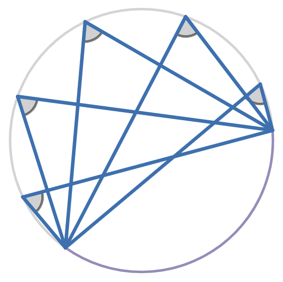
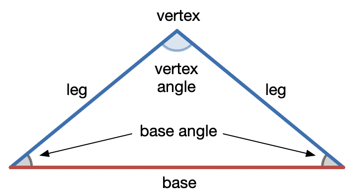
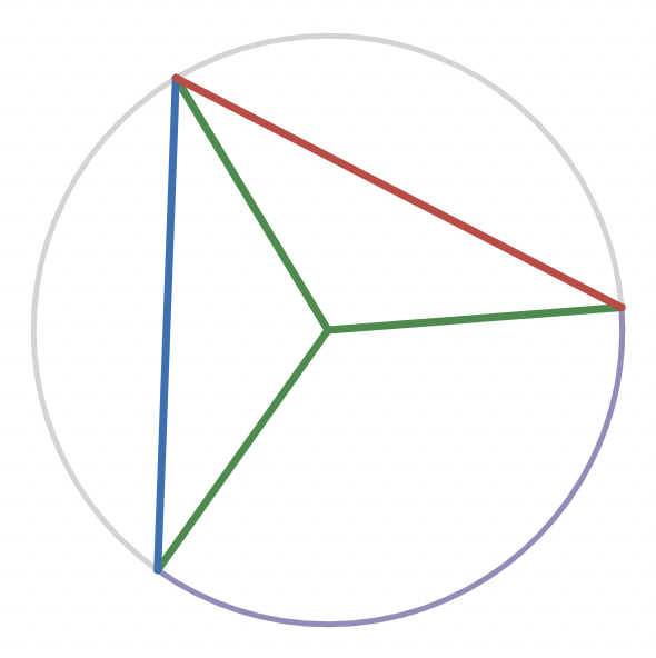
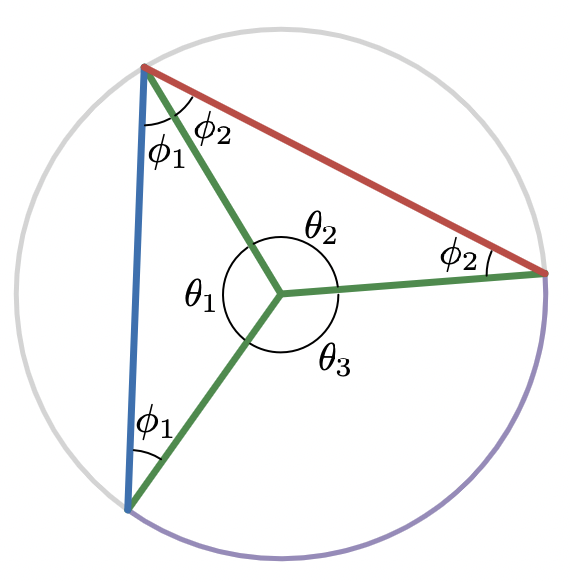
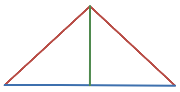
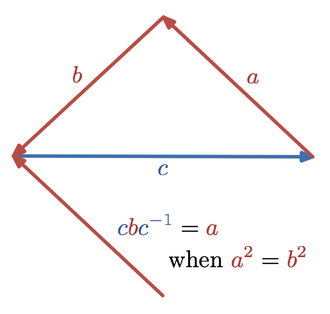
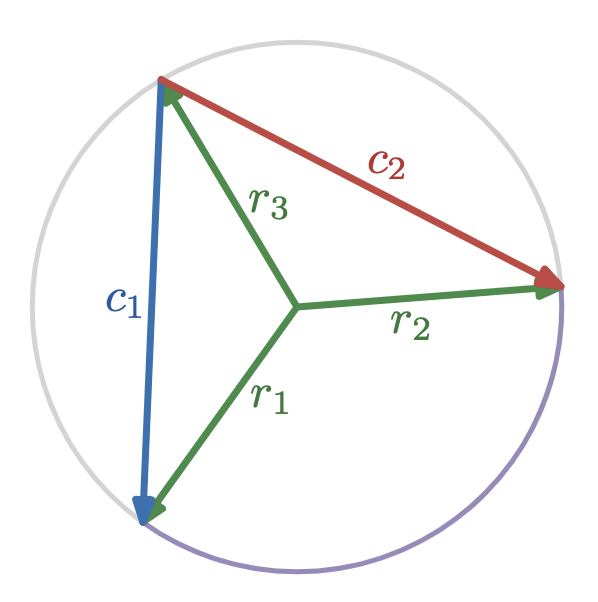
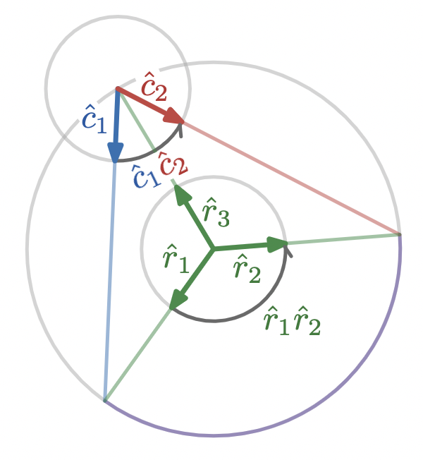
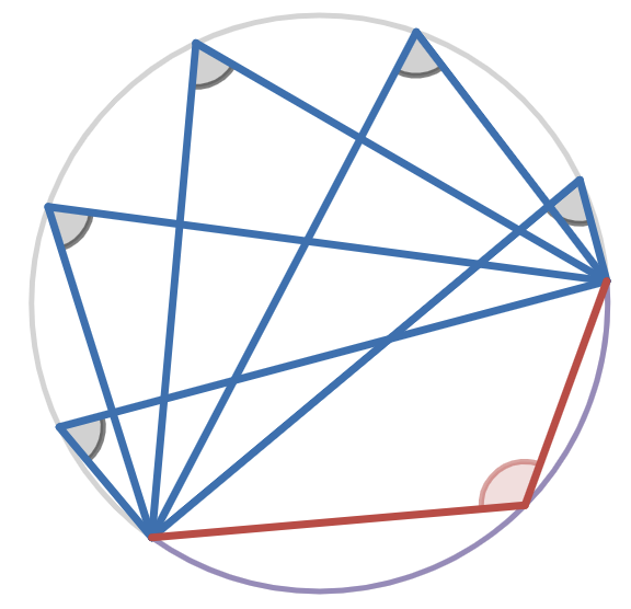
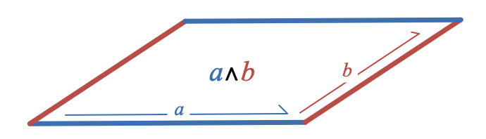
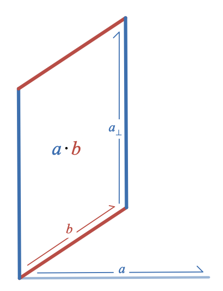
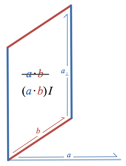
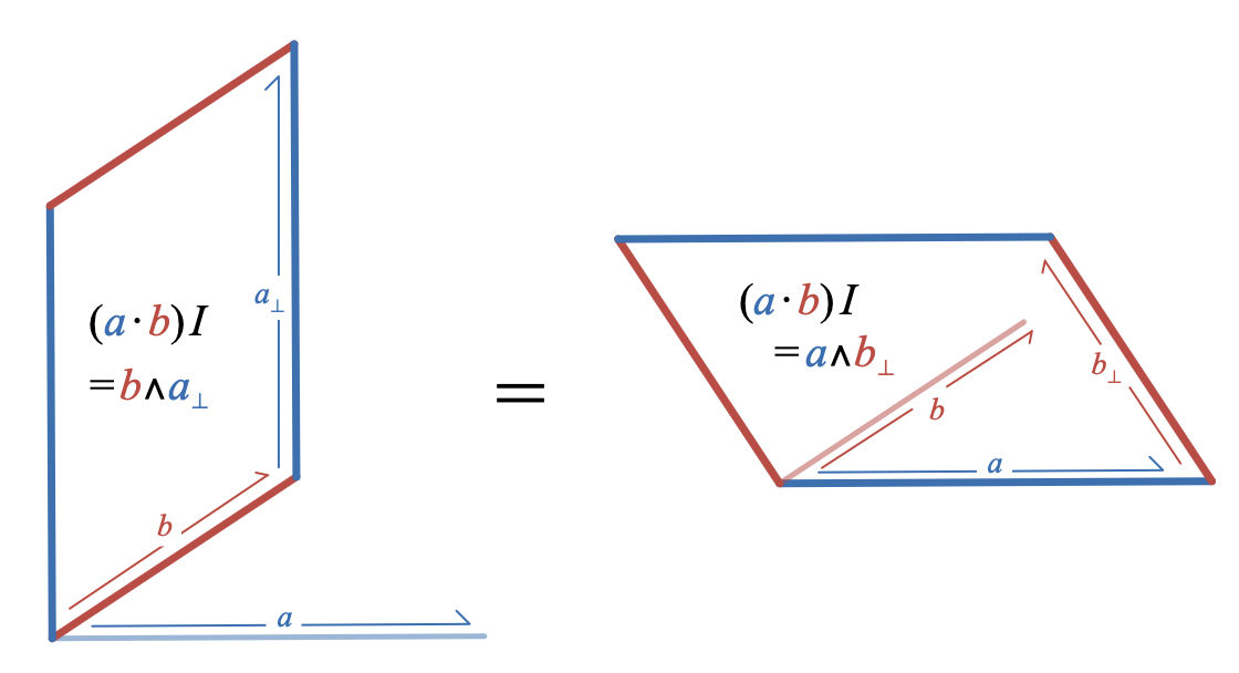
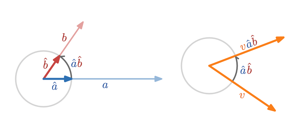
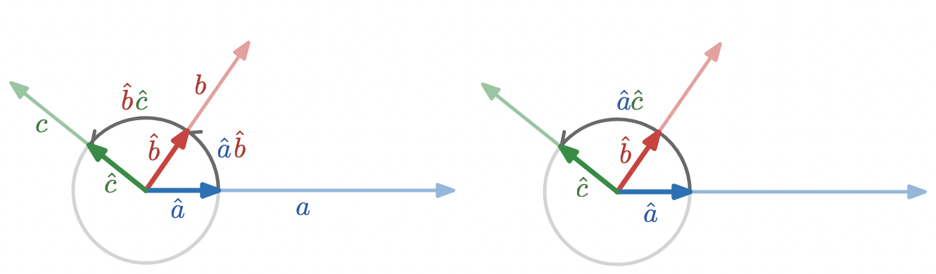 \begin{aligned} (\hat{a} \hat{b}) (\hat{b} \hat{c}) &= \hat{a} \hat{b} \hat{b} \hat{c} \\ &= \hat{a} (\hat{b} \hat {b}) \hat{c} \\ &= \hat{a} \hat{c} \end{aligned}
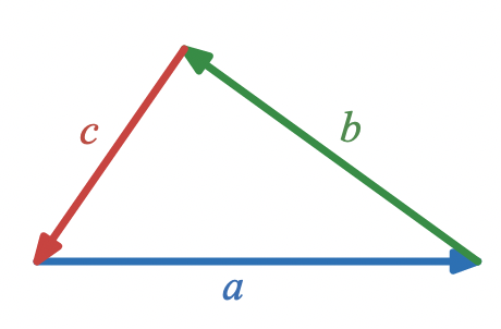
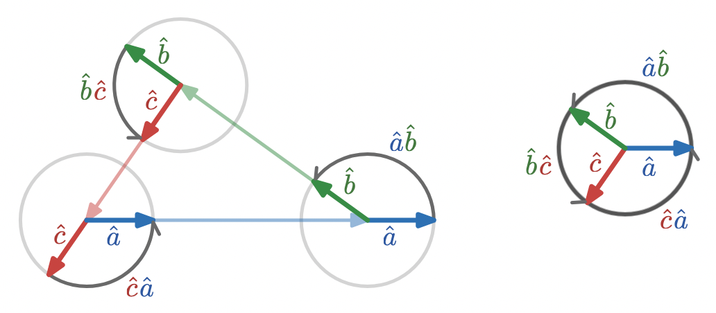
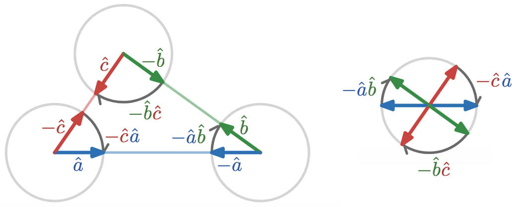 \begin{aligned} &(-\hat{a} \hat{b})(-\hat{b} \hat{c})(-\hat{c} \hat{a}) \\ &= - \hat{a} \hat{b} \hat{b} \hat{c} \hat{c} \hat{a} \\ &= -1 \end{aligned}
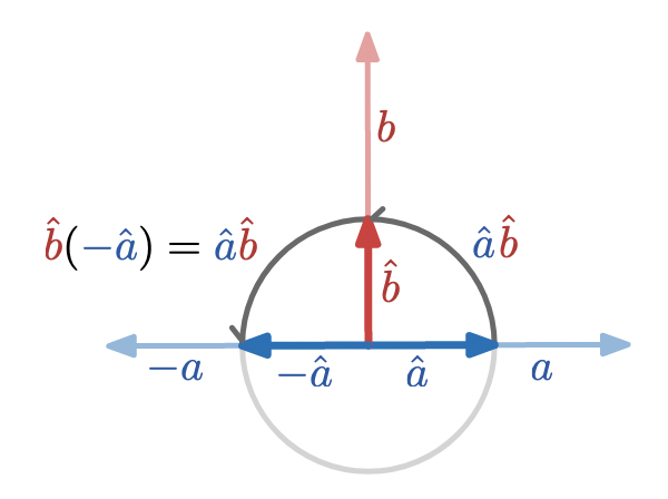
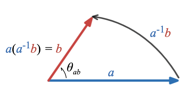
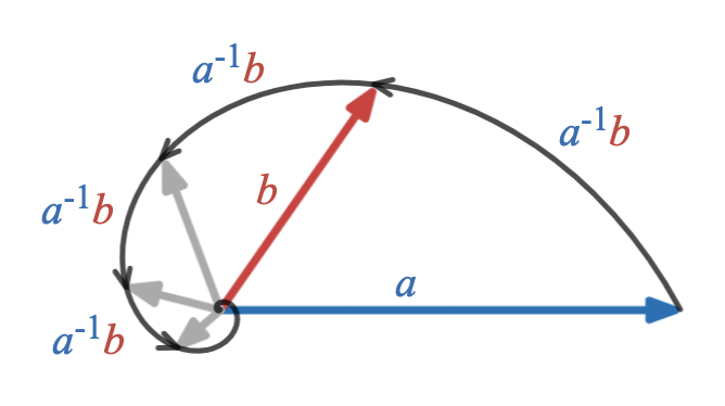
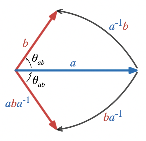
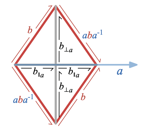
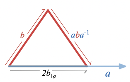 b_{\parallel a} = \frac12 \left(b + aba^{-1}\right)
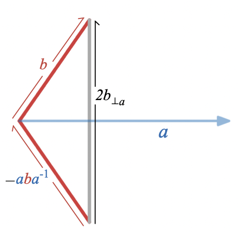 b_{\perp a} = \frac12 \left(b - aba^{-1}\right)
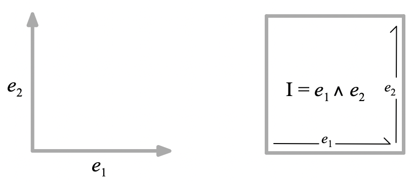
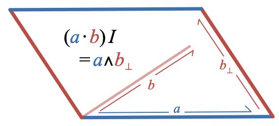 (a \cdot b) I = a \wedge b_\perp
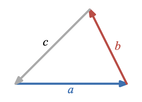
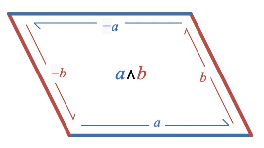
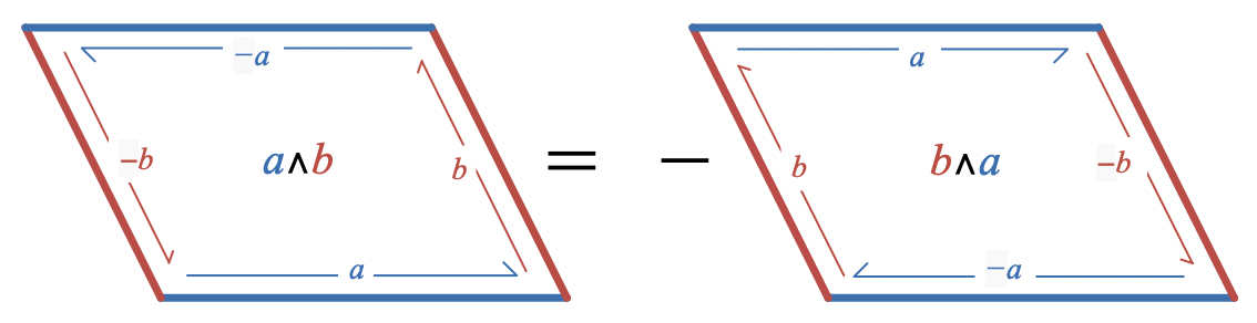
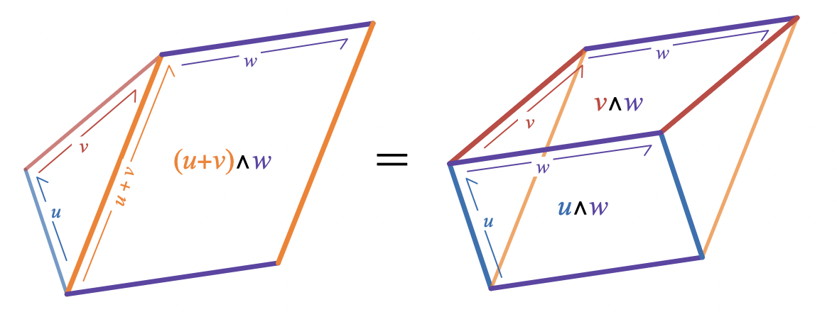

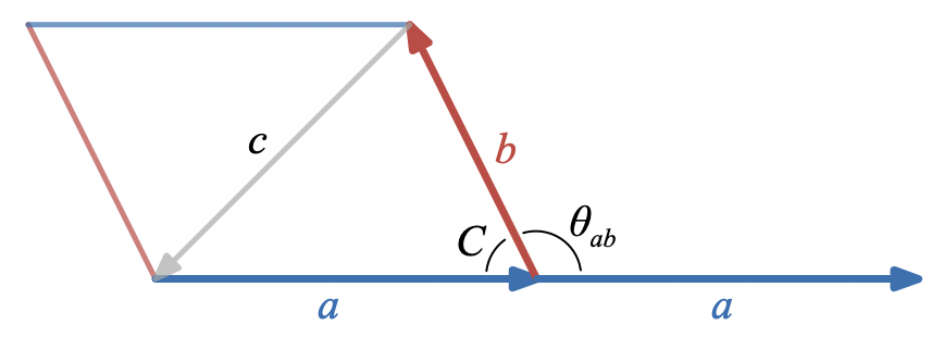
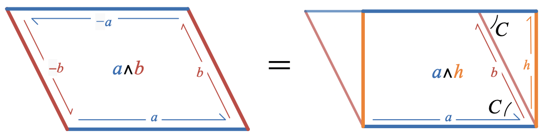
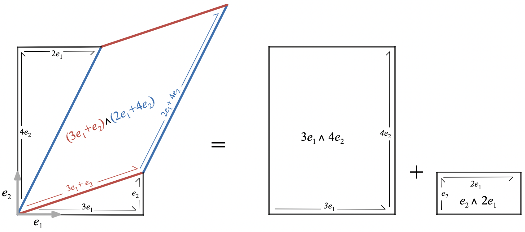
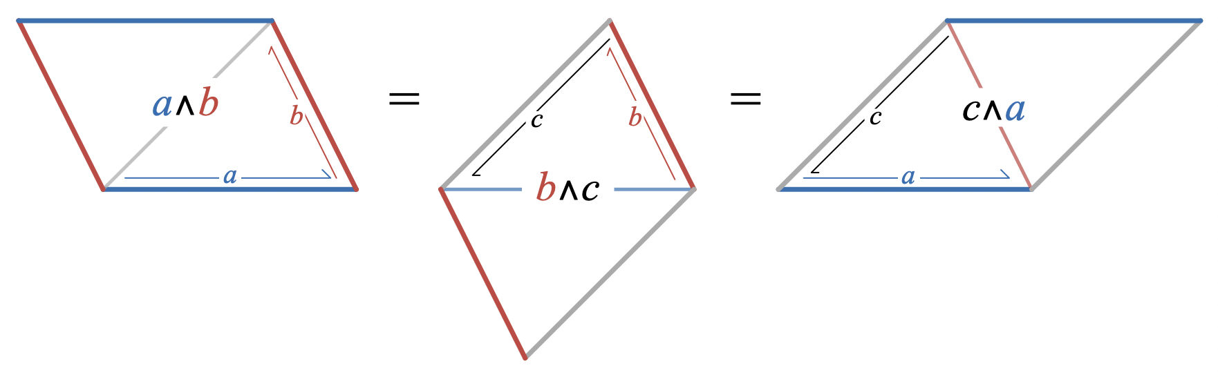
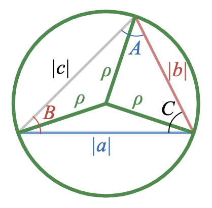
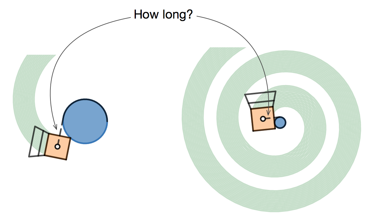
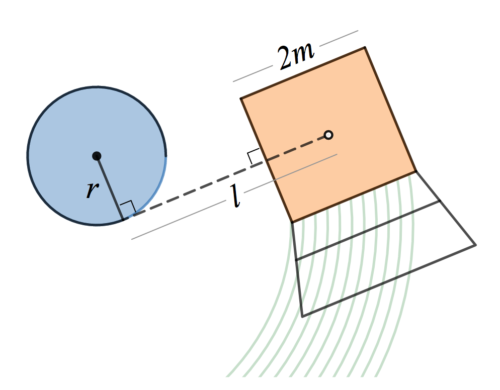
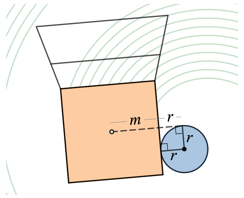
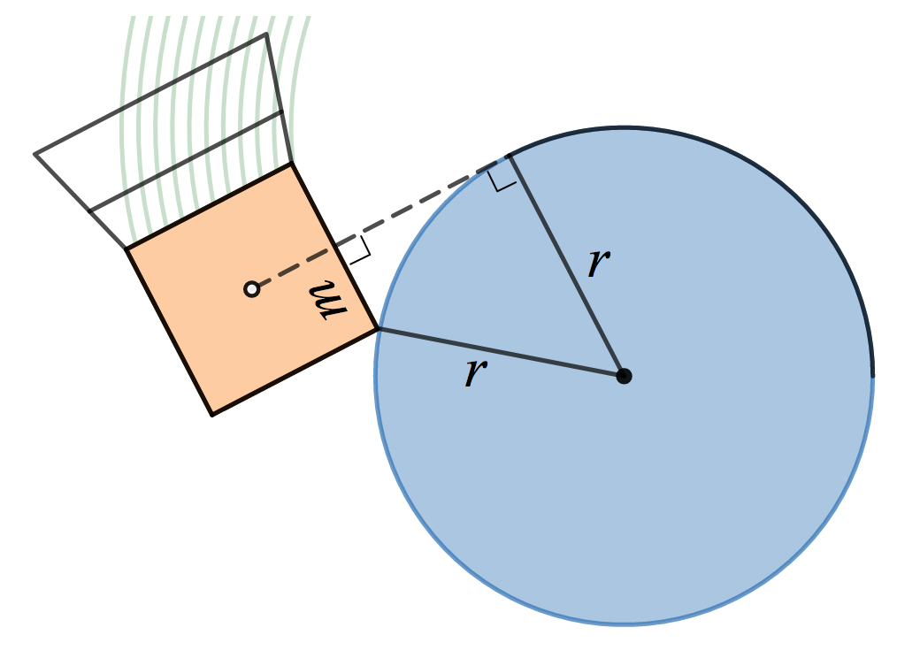
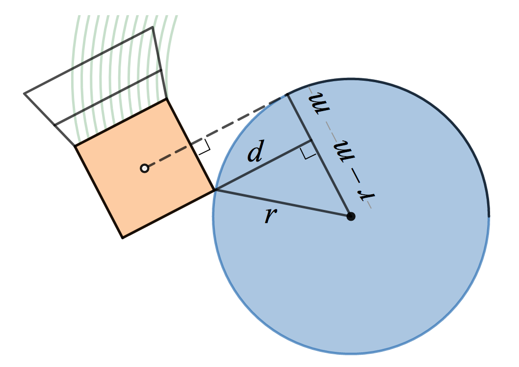
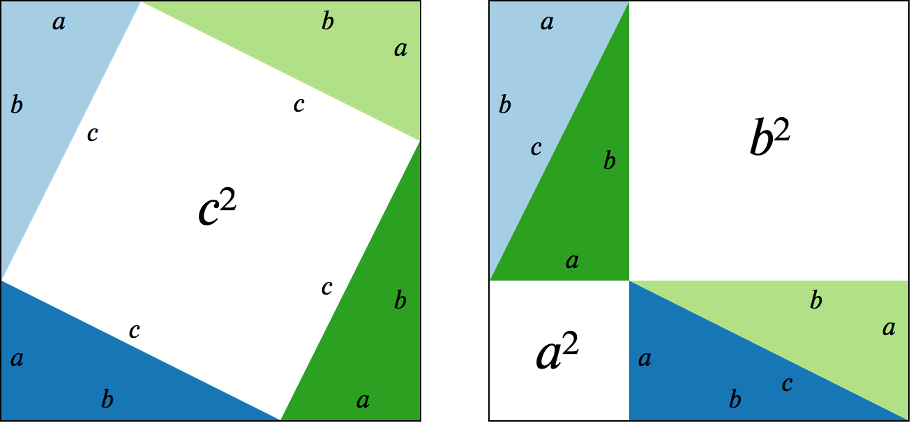
In the angle form, is an interior angle, but in the vector form, if , then is an exterior angle. This is the origin of the difference in sign of the final term between the two forms. . If you have a theorem about right triangles, then you’d really like to know whether it’s ever true for non-right triangles, and how exactly it breaks down in cases where it isn’t true. Perhaps there’s a good way to deform Pythagoras’ picture to illustrate the law of cosines, but I don’t believe I’ve seen it.
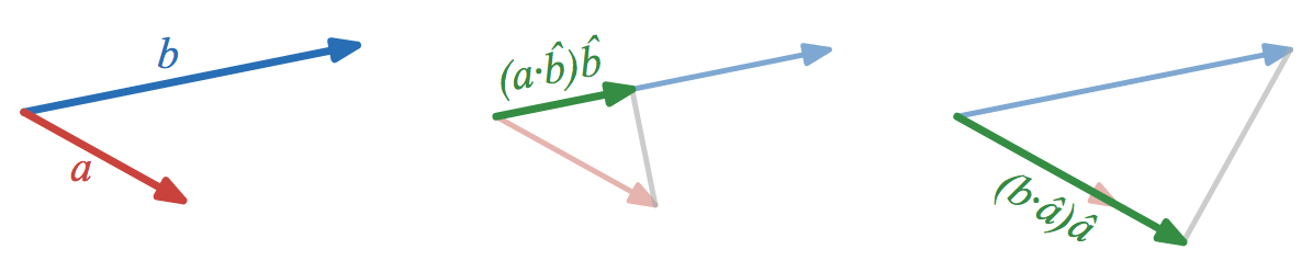
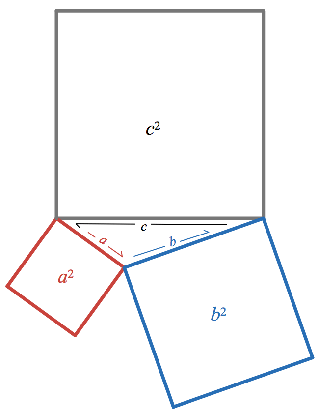
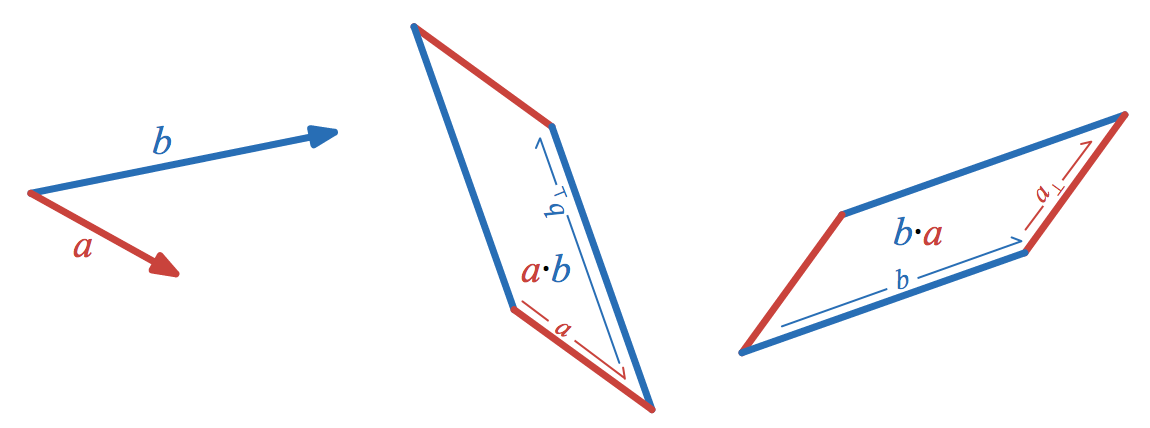
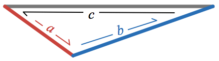
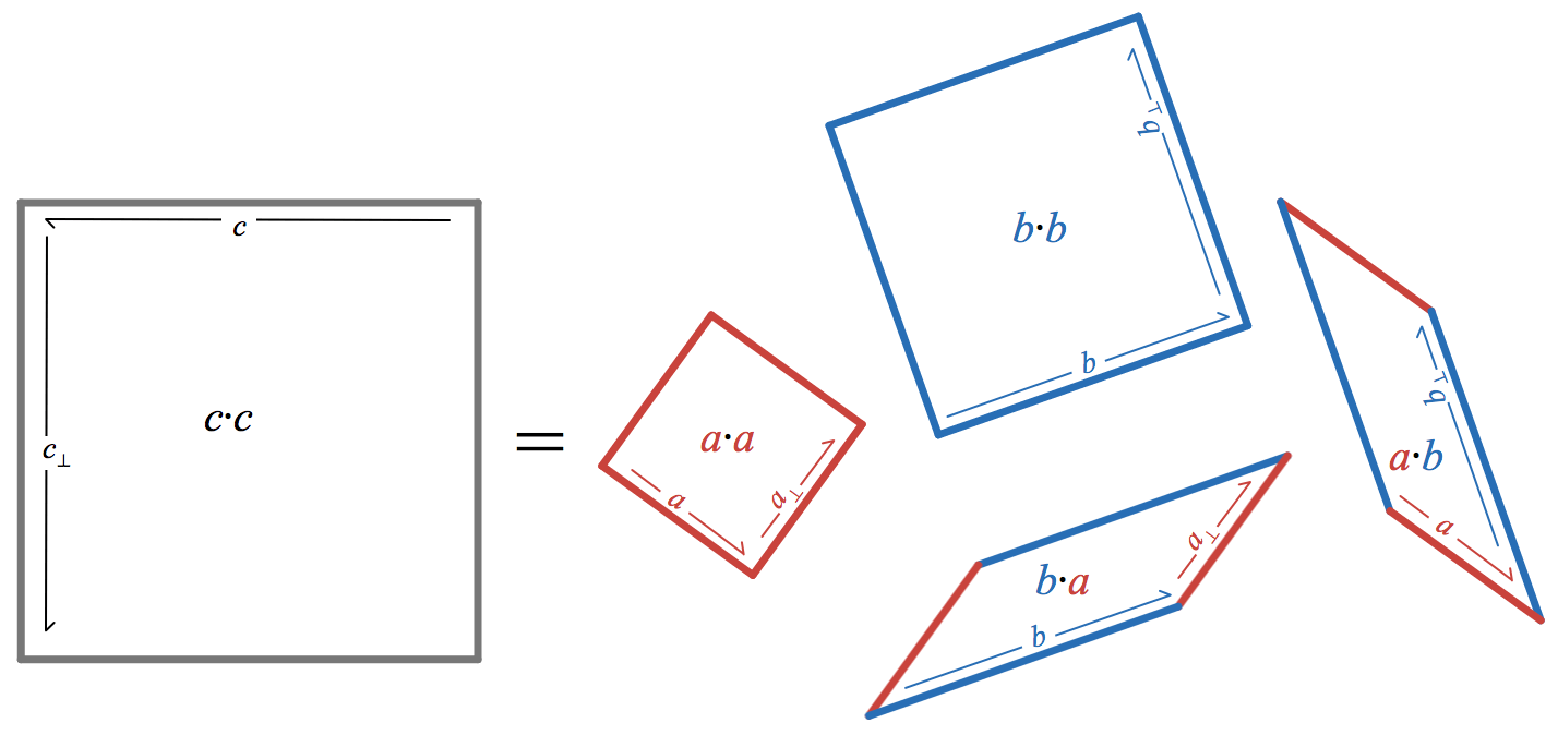
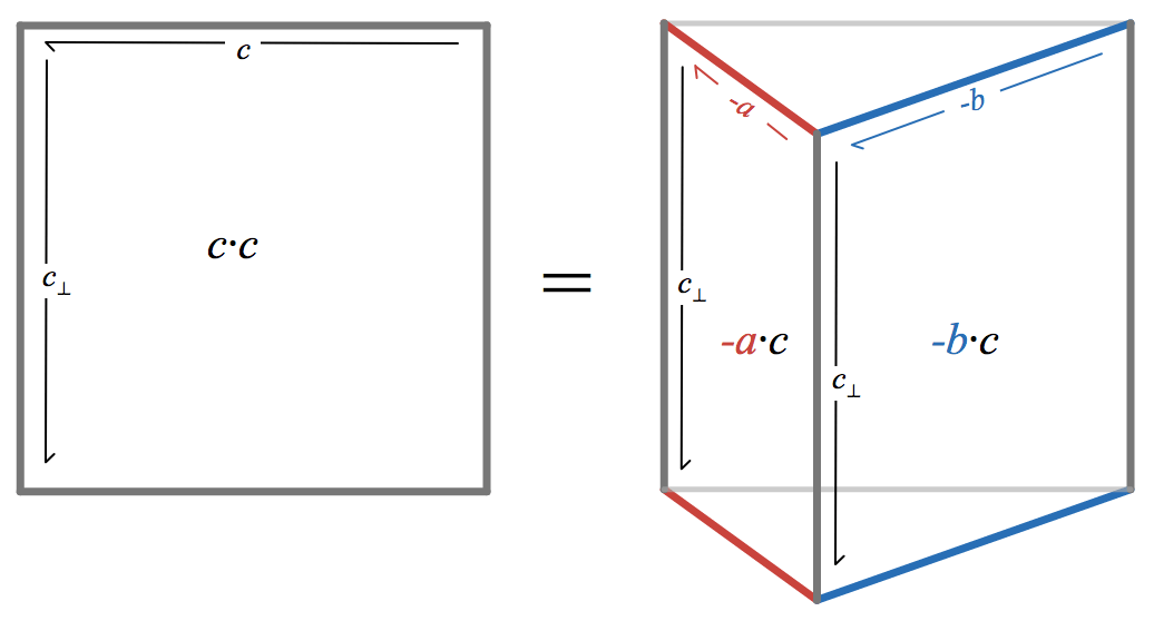
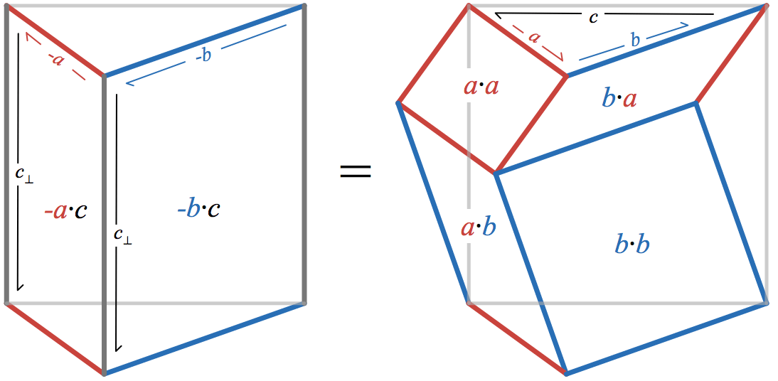
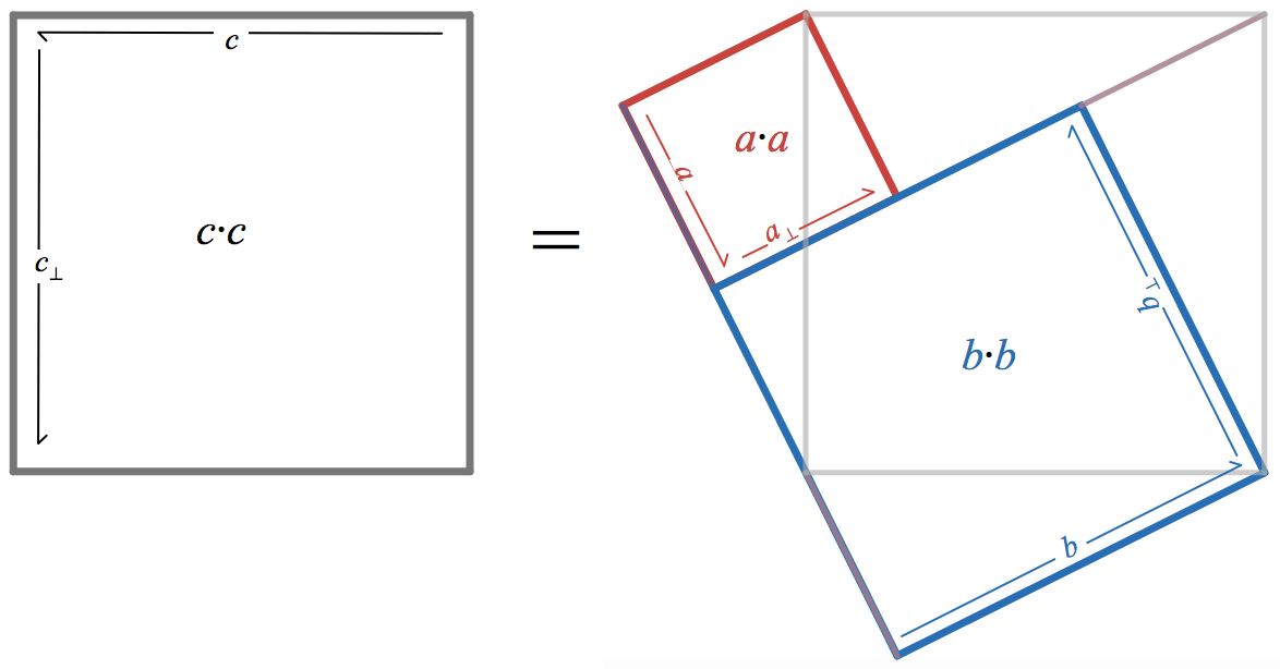
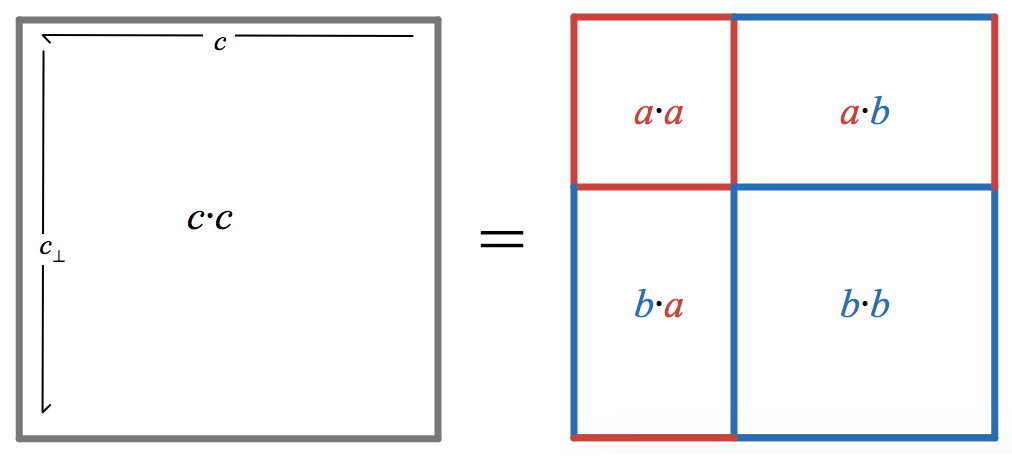
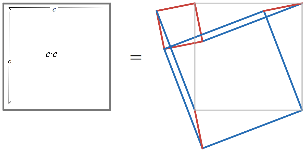